Sizing Up Your ScyllaDB Cluster

Update: We recently created the following video to explain what matters most when building a cluster for your workload.

***

There was a time when high node counts conferred bragging rights. “You’ve only got 500 nodes of Cassandra? Well we run 5,000 nodes, and we like it!” That was then; this is now. Node sprawl is a real problem in today’s datacenters. It’s a problem for developers, administrators, and the bean counters. Also known as ‘wasteful overprovisioning,’ node sprawl often reflects an effort to spend your way to low latency and high availability. What’s even worse is that all the overspending might not even meet the performance requirements anyway.

It’s hard to break out of this mentality. After all, overprovisioning can provide a cushion (albeit an expensive one) against traffic spikes, outages, and other forms of mayhem. But that comes at the cost of more server failures and higher administrative overhead.

There is a good chance that your team selected ScyllaDB in part because it leverages all of the computing power available in modern hardware. That means lower costs, far less operational interaction, and smaller clusters—less waste overall. Rather than overprovisioning, you’re instead running at the highest levels of utilization possible.

In practical terms, how do you begin to plan your ultra-efficient ScyllaDB topology? The shift can be intimidating for those coming from a background in Cassandra, or for those coming from a primary-replica architecture, or from a plain old monolithic database implementation.

In this post we’ll layout a checklist for designing a ScyllaDB cluster that incorporates both horizontal and vertical scaling.

Dimensions of Scale

When you are designing systems to handle large data, you have a few primary considerations and also a number of secondary considerations.

Primary Considerations

• Storage
• CPU (cores)
• Memory (RAM)
• Network interface(s)

These are the most readily-apparent and predictable sizing elements. Especially storage. For ScyllaDB, there are already some assumptions in 2019: your storage will be NVMe SSDs. (Long gone are the days when people are willing to take the latency hits for spinning HDDs.) Not only do you need to size your disks for basic data, you also need to calculate total storage needed based on your replication factor, as well as overhead to allow for compactions.

Next is the CPU. As of this writing, you are probably looking at modern servers running on Intel Xeon Scalable Processor Platinum chips, such as the E5-2686 v4 (Broadwell) which operate at 2.3 GHz speeds, or something in that range. These can be found commonly across AWS, Azure, and Google Cloud. You will need to size your server needs based upon how much throughput each of these multicore chips can support.

Random Access Memory (RAM) is your third consideration. ScyllaDB is performant by leveraging the internal data cache, memtables and, in ScyllaDB Enterprise, in-memory tables. You need to ensure that your system can support a sufficient disk-to-memory ratio, or you will be hitting your storage far more than you probably want if you wish to keep your latencies low.

Lastly, you have to ensure that network IO is not your bottleneck. Most of the time you have no choice. NICs are generally not a configurable option on a public cloud node, but you should keep it in mind because it could turn into a gating factor. For one salient example, the new Amazon EC2 i3en.24xlarge node, which can pack up to 60 TB of storage also sports a 100 Gbps network interface. You can read about our analysis of this large node here.

Storage: How Big is Your Dataset, and How Fast is it Growing?

ScyllaDB users run datasets ranging from tens of gigabytes to greater than a petabyte. Data resilience depends on the number of replicas stored in ScyllaDB. The most common topology involves 3 replicas for each dataset, that is, a single cluster with a replication factor of 3 (RF=3).

We will use that replication factor in the examples that follow. When referring to raw data size, we refer to data size before replication. With this in mind, let’s take the following example and start our sizing exercise.

Your company has 5TB of raw data, and would like to use a replication factor of 3.

5TB Data X 3 RF = 15TB

You should plan to initially support 15TB of total data stored in the cluster. However, there are more considerations we must understand.

Data Over Time

15TB is only a starting point, since there are other sizing criteria:

• What is your dataset’s growth rate? (How much do you ingest per hour or day?)
• Will you store everything forever, or will you have an eviction process based on Time To Live (TTL)?
• Is your growth rate stable (a fixed rate-of-ingestion per week/day/hour) or is it stochastic and bursty? The former would make it more predictable; the latter may mean you have to give yourself more leeway to account for unpredictable but probabilistic events.

You can model your data’s growth rate based on the number of users or end-points; how is this number expected to grow over time? Alternately, data models are often enriched over time, resulting in more data per source. Or your sampling rate may increase. For example, your system may begin ingesting data every 5 seconds rather than every minute. All of these considerations impact your data storage volume.

So rather than just design your system for your current data, you may wish to provision your system for where you expect to end up after a certain time span. For ScyllaDB Cloud, or ScyllaDB running on a public cloud provider, you won’t need that much lead time to provision new hardware and expand your cluster. But for an on-premises hardware purchase, you may need to provision based on your quarterly or annual budgeting process.

Make space for compaction

The compaction process keeps the number of internal database files to a reasonable number. During the compaction process, ScyllaDB needs to store temporary data. When using the most common compaction strategy, known as Size Tiered Compaction Strategy (STCS), you need to set aside the same amount of storage for compaction as for the data, effectively doubling the amount of storage needed.

Resulting in:

5TB (of raw Data) x 3 (for RF) x 2 (to support STCS) = 30TB

So, 30TB of storage is needed for this deployment, assuming there will not be a significant increase in your dataset in the near future. You will have to divide this total amount across your cluster size. So, for example, 3 nodes of 10TB each; or alternately 6 nodes of 5TB each.

Throughput: Data Access Patterns

Data is rarely at rest in the cluster! User applications are adding, deleting, modifying and reading all that data. These access patterns have a direct impact on your cluster sizing.

The data persisted into ScyllaDB is entered in append only mode. That means that from a sizing perspective all data mutations are considered to be the same operation. Reads use a different data path when retrieved.
Workloads might have different write and read rate, applications require different adherence to latency

For this example we’ll use the following workload and access pattern for a hypothetical application:

• A “mostly write” workload of 70,000 writes per second and 30,000 reads per second, resulting in a total of 100,000 operations per second.
• Application developers require that, under a maximum load of 100,000 transactions per second:
  • Writes 99th percentile: ≤10 milliseconds
  • Reads 99th percentile: ≤15 milliseconds
• Payload per transaction is expected to be 1Kbyte or less

As maintainers of the system, we will need to create a system that is utilizing our resources properly, while supporting the required throughput at the set of latency.

Keep the above information in mind, we will use it in our sizing exercise.

Counting cores

ScyllaDB is unique in its ability to maximize the power of modern, multi-core processors. For that, core count is an important consideration. Today, servers with 8 physical cores or more are common in both on-prem and cloud deployments. Generally speaking, for payloads under 1 kilobyte, ScyllaDB can process ~12,500 operations per second for each physical core on each replica in the cluster.

To translate the above example to number of cores:

• 100,000 OPS *1KB (payload) * 3 (Replicas) = 300,000 OPS
• 300,000 OPS / 12,500 (operations/core) = 24 physical cores (or 48 hyperthreads)

Using servers with 8 cores each, we end up with 3 servers needed for deployment.

In many cloud deployments, nodes are provided on a vCPU basis. The vCPU is typically, a single hyperthread from a dual hyperthread x86 physical core. ScyllaDB shards per hyperthread (vCPU). Translating the above 24 physical cores to vCPUs will result in 48 vCPUs.

Use the following formula (for Intel Xeon Scalable Processors):

• (Cores * 2) = vCPUs available for shards

A note on interrupts

ScyllaDB likes to use CPUs for processing users’ requests and less for handling out-of-flow code. To minimize interrupts from network devices and other hardware system, ScyllaDB designates threads to be dedicated for interrupt handling. In your ScyllaDB deployment you will see that ScyllaDB will not assign two or more threads to its consumption; these threads will be dedicated for interrupt handling. In case you have less than 8 threads in the ScyllaDB server, ScyllaDB will not be assigning threads for interrupts, and all interrupt handling will shared among available threads.

Solving for Latency

You have two types of latency when you design distributed database systems: internal latency and end-to-end (or round-trip) latency. Internal latency is the delay from when a request is received by the database (or a node in the database) and when it provides a response. End-to-end (or round-trip) latency is the entire cycle time from when a client sends a request to the server, and when it obtains a response.

The internal latency is dependent on your system building blocks: CPU, Memory and Disk I/O. Each of these could be a potential point of bottlenecking.

When the requirement exists for low latency—as in the example above ≤10ms for writes and ≤15ms for reads—the system building block should have adequate performance to meet these requirements. For the write latencies, an ample amount of CPU is needed to process the transaction, and fast disk I/O system to persist the data insertion or mutation. For fast reads, In addition to CPU and fast disk I/O system, a sizable internal cache will help meeting the latency requirements. ScyllaDB’s internal caching layer efficiency is dependent on the amount of memory a ScyllaDB node has. We will discuss the memory importance in this document below.

The end-to-end latency is dependent on factors that might be outside of ScyllaDB’s control, for example:

• Multi-hop routing of packets from your client application to the ScyllaDB server, adding 100’s of milliseconds in latency.
• Client driver settings, connecting to remote datacenter
• Consistency levels that require both local and remote datacenter responses
• Poor network performance between clients and ScyllaDB servers.

Accounting for all the above variables requires understanding of the deployment architecture, application and ScyllaDB servers. ScyllaDB recommends placing your application servers as close as possible to the ScyllaDB servers. Set your client connection to the local datacenter, and use Local_Quorum, Local_One etc as your consistency level settings.

From a network hardware perspective, a 10Gbps+ network is the recommended network infrastructure.

The importance of memory

ScyllaDB will utilize memory to store your database data. RAM access (measured in tens of nanoseconds) is about three orders of magnitude faster than disk access (measured in tens of microseconds). ScyllaDB needs RAM for a number of purposes: for data cache, for memtables, and, if you are using ScyllaDB Enterprise, for in-memory tables.

ScyllaDB will allocate roughly 50% of your server memory to establish an internal caching system. This caching system will help your application’s data retrieval. A repetitive read of data can be very efficient if it is stored in server memory. ScyllaDB deploys a Least Recently Used (LRU)-based caching system to store the latest data read from the SSTables. If the data has not changed between consecutive reads of the same data, the second and subsequent times can be read from the caching layer, saving the laborious process of re-reading the information from files stored on disk.

The larger the memory a machine has, the larger the cache size ScyllaDB can create, and thus the higher probability the data you are searching for is stored in server memory.

For ScyllaDB, the minimum required RAM is 1GB per core. For highly-repetitive read workloads ScyllaDB recommends increasing RAM to the largest that is economically possible.

We recommend 30:1 as the optimal ratio of Disk:RAM size ratio and a maximum of 80:1 Disk:Ram ratio. In other words, for a 20TB storage in your node, we would recommend at least 256GB RAM, and preferably closer to 666GB RAM.

Also, if you do use in-memory tables, we recommend that you ensure that no more than 40% of that reserved memory be utilized by in-memory table data; the other 60% will be used for compactions (read more about this feature in our documentation). Beyond the memory you reserve for the in-memory table you must still ensure that you have at least 1GB of RAM per node left over to support data cache and memtables.

Do you need multi region or global replication?

When you start deploying a distributed database across regions or continents, you start incurring network delays. And the ultimate network delay is the speed of light itself; a hard limit to the propagation of information.

A key concern is whether your business needs to support a regional or global customer base. By putting ScyllaDB clusters close to your customers, you lower network latency. You can also improve availability and insulate your business from regional outages.

Creating a multi data-center deployment is a simple task with ScyllaDB.

ScyllaDB’s recommendation is to keep a homogeneous deployment in terms of node sizes and datacenter sizes.

The following graphic shows the concept of datacenter replication. While the two data-centers are independent in terms of responses to clients, the data-centers are still considered a single ScyllaDB cluster, relating to a single cluster name.

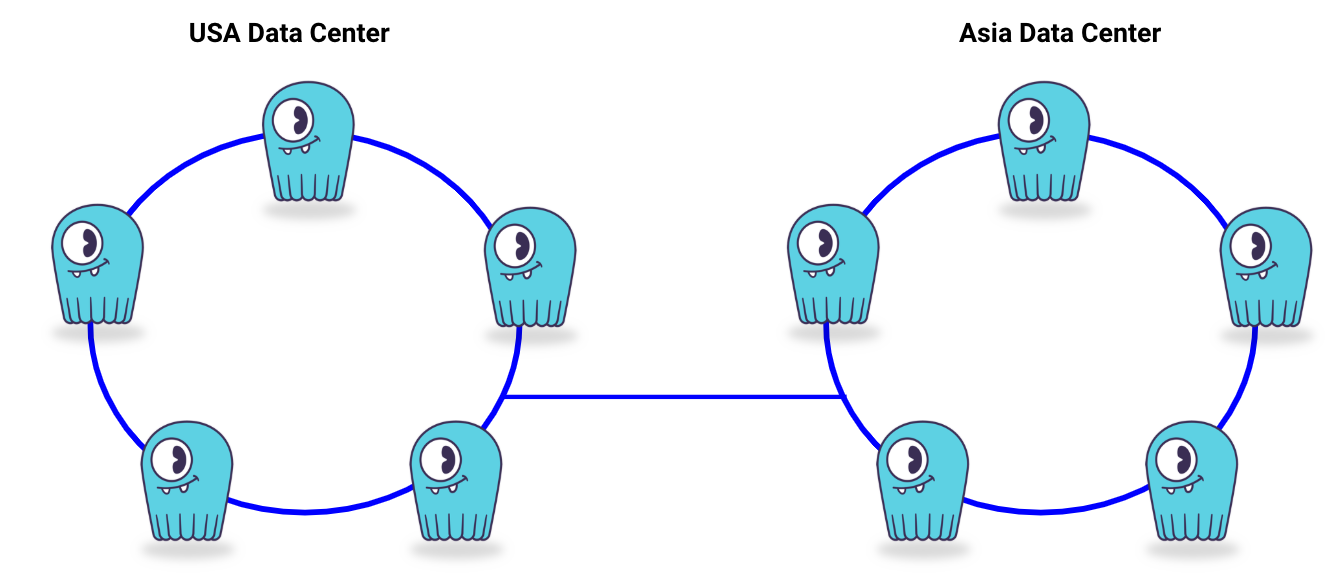
Ok, so how do I make sure data is replicated between clusters?

That part is easy, you will need to declare which data-centers data should be replicated to, on a per keyspace definition. Here is an example:

CREATE KEYSPACE appdata WITH replication = {'class': 'NetworkToplogyStrategy', 'usa’: '3', ‘asia’: ‘3’}

The above example create three replicas per data-center, resulting in a total of 6 replicas in the cluster for the keyspace named: appdata.

Application clients may or may not be aware of the multi datacenter deployment, and it is up to the application developer to decide on the awareness to fallback data-center(s). The settings on load balancing are within the specific programing language driver.

Multi Availability Zones Vs Multi region

Today, Infrastructure as a Service (IaaS) providers offer various highly available deployment options. To mitigate a possible server or rack failure, IaaS vendors offer a multi zone deployment. Think about it as if you have a data center at your fingertips and you can deploy each server in its own rack, using its own power, top-of-rack switch and cooling system. Such deployment will be bulletproof for any single system failure, as each rack is self-contained.
The availability zones are still located in the same IaaS region. However, a specific zone failure should not affect other zones deployed servers.

For example on Google Compute Engine: us-east1-b, us-east1-c and us-east1-d availability zones are located in the us-east1 region (Moncks Corner, South Carolina, USA). But, each availability zone is self contained. Network latency between AZs in the same region is negligible for the purpose of our discussion.

In short, both Multi Availability Zone and Multi-region deployments will help with business continuity/disaster recovery, but multi-region has the additional benefit of minimizing local application latencies in those local regions.

Network interface

Data has to make its way to and from the ScyllaDB server. In addition, replication of data among the scylla servers, backend processes such as repair and node recovery, requires network bandwidth to move data.

Most IaaS vendors provide a modern network system providing ample network bandwidth between your ScyllaDB servers and between ScyllaDB and the application client servers. As of mid-2019 commonly-available datacenter-grade network interfaces run at 10Gbps. Plus there are some rarer high-end devices that operate at 100Gbps (such as the i3en.24xlarge on AWS EC2).

The following is iperf output from the network bandwidth between two Google Compute Engine (GCE) servers:

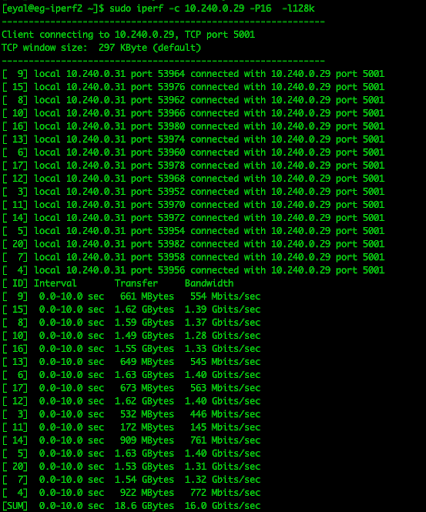
By this, you can see that traffic commonly exceeds gigabit per second levels. The recommendation from ScyllaDB is to provide at least a 10Gbps network interface between your servers in order to make sure that the network does not bottleneck the performance of your database.

Last but not least, Monitoring

When deploying ScyllaDB you can see using ScyllaDB Monitoring Stack how your applications and database behave under load. ScyllaDB Monitoring Stack utilizes Prometheus and Grafana to store and visualize the metrics, respectively.

This step is to ensure that your calculations were correct, or at least close. It is helpful for your developers to know that with a good data model design they can achieve lower latency when reading from cache instead of reading from disk. It is also important to the database maintainer to know if she over-provisioned or under-provisioned the system.

To deploy ScyllaDB monitoring you will need an additional server which can connect to the ScyllaDB cluster using ports 9100 and 9180; the monitoring prometheus server is exposed over port 9090 and the Grafana dashboards are visible on port 3000.

Here is the recommendation for the monitoring server specification:

• CPU: at least 2 physical cores (4 vCPUs)
• Memory: 15GB+
• Disk: persistent disk storage proportional to the number of cores and Prometheus retention period (see the following section)
• Network:1GbE to 10GbE preferred

Calculating Prometheus Disk Space requirement

Prometheus storage requirements are proportional to the number of metrics it holds. The default retention period is 15 days, and the disk requirement is around 200MB per core.

For example, when monitoring a 6 node ScyllaDB cluster, each with 16 cores, and using the default 15 days retention time:

6 (nodes) * 16 (cores per node) * 200MB (of data per core) = ~20GB

To make it sustainable for possible growth in cluster we’d recommend a minimum of 100GB drive for the Prometheus storage. The larger the number of total ScyllaDB cores you deploy the larger the Prometheus storage should be.

Translating numbers to real-world platforms

Let’s get back to our example sizing. As a reminder an application generates the following workload, plus some new considerations (marked in red below):

• 70,000 writes per second and 30,000 reads per second, resulting in a total of 100,000 operations per second.
• Application developers require that, under a maximum load of 100,000 transactions per second:
  • Writes 99th percentile: ≤10 milliseconds
  • Reads 99th percentile: ≤15 milliseconds
• Total data stored in the next 12 months: 1.5TB raw data
  • Replication factor: 3
  • Using SizeTieredCompactionStrategy
  • Total storage required: 9TB
• Single Datacenter deployment

Let’s deploy ScyllaDB on Amazon Web Services

Of all AWS instances, the i3 family is the most compelling for ScyllaDB deployments. The large and powerful ephemeral storage system associated with these instances provides for an efficient and highly scalable ScyllaDB cluster.

We will be using 3 nodes of i3.4xlarge for ScyllaDB deployment. Each i3.4xlarge has 16 vCPUs, 122GB of RAM and 3.8TB of NVMe based data storage. That gives us a total of 48vCPUs and 11.4 TB of disk storage.

We will be using a single node of m5.xlarge for ScyllaDB monitoring with 100GB of EBS volume.

Now let’s see if our deployment can meet above requirements:

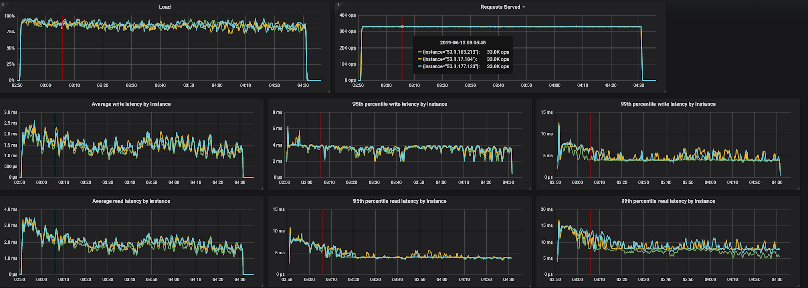
The above image is from the ScyllaDB monitoring system, monitoring a 3 node cluster of i3.4xlarge servers on AWS US-EAST-1, under the above described load, modeled using Cassandra-Stress tool, Using the following command deployed on three identical, independent client machines:

cassandra-stress mixed ratio\(write=7,read=3\) duration=100m cl=QUORUM -schema "replication(factor=3)" -mode native cql3 connectionsPerHost=10 -col "n=fixed(5) size=fixed(206)" -pop "dist=gaussian(1..200000000,100000000,30000000)" -rate threads=800 throttle=33000/s -node $NODES

• Top left chart (Load) shows the ScyllaDB servers utilization.
• Top right chart (Requests Served), shows the number of requests each server handles, each server hands ~33K operations per second, totaling in 100K operations per second for the datacenter.
• Middle charts are (left to right): the average, 95% and 99% write latency metrics as they are measured at the ScyllaDB server edge.
• Bottom charts are (left to right): the average, 95% and 99% read latency metrics as they are measured at the ScyllaDB server edge.

The above deployment meets the criteria of throughput and latency. However, the deployment does not take into account maintenance windows, possible node failures and fat-finger errors. To be on the safe side, and to be able to maintain the workload at ease in case of any mayhem, we’d recommend at least 4 nodes of i3.4xlarge.

In case you deploy ScyllaDB in a multi Availability Zone (AZ) environment, the recommendation would be to have identical number and size instances in each AZ. For the above example we will have 2 options of deployment in a 3 AZ scenario:

• 2 nodes of i3.2xlarge in each AZ, which will provide exact performance as described but without any cushioning for node failure.
• 2 nodes of i3.4xlarge in each AZ, which will provide ample amount of resources to sustain a full AZ failure

Please note, AWS charges network traffic cost for data streaming between availability zones in the same region. With RF=3 it means you network cost for inter-AZ communication is 3x higher than in the case you’d deploy in a single AZ. AWS does not charge network traffic for same AZ communication.

ScyllaDB on Google Compute Engine

Deploying ScyllaDB on Google Compute Engine will follow similar steps and number of instances as we would use on AWS.

Looking into Google Compute Engine (GCE) instance catalog, we found the following instances to meet the workload demand:

• Deploying in a Single AZ: 3x n1-standard-16 with 3TB of NVMe ephemeral storage
• Deploying a multi AZ using 3 AZs:
  • 2 nodes of n1-standard-8 with 1.5TB of NVMe Drive, per AZ. Providing the exact amount of resources without any room for node failure.
  • 2 nodes of n1-standard-16 with 1.5TB of NVMe Drive per AZ. Providing ample amount of resources for node or full AZ failure.

ScyllaDB On-Premises

With on-prem deployment (and we’ll use that term whether actually on-premises or in an offsite colocation facility) we have a more flexible server configurations. We recommend at least 3-node deployment using 16 physical core servers, with SSDs (preferably NVMe based) data storage devices.

For the above use case we will select 3 servers, each using a dual socket server populated with 2 CPUs, 8 cores each (e.g. intel Xeon E5-2620 v4), 128GB of RAM and total of 3TB NVMe drives (e.g. 2x Samsung PM1725 MZWLL1T6HAJQ cards), 10Gbps network card, dual power supply.

Hey! which operating systems do you support?

ScyllaDB is supported on the major Linux distributions. We support RHEL, CentOS, Ubuntu, Oracle Linux and Debian Linux operating systems. Please refer to the following page for the most updated information on supported operating systems.

OK! You got the size of cluster you need, what’s next?!

So, you read through this long journey and you’d like to get your feet wet. There are several options you can jump start your evaluation of ScyllaDB:

• Download and install ScyllaDB into your favorable infrastructure (on-prem or public cloud), test your workload.
• Or get started immediately with ScyllaDB Cloud (NoSQL DBaaS), our fully managed ScyllaDB Enterprise grade service. Instances are deployed on powerful AWS i3 family instances. With a few clicks you can get your ScyllaDB cluster going at your favorable geo-region. Find out more here.

If you already started testing ScyllaDB, let us know how you are doing. We enjoy learning about new and innovative use cases. We’d love to hear what worked and what barriers you still face. Sometimes a small Slack chat can leapfrog your progress.