“Now, here, you see, it takes all the running you can do, to keep in the same place. If you want to get somewhere else, you must run at least twice as fast as that!” — The Red Queen to Alice, Alice Through the Looking Glass
In the world of Big Data, if you are not constantly evolving you are already falling behind. This is at the heart of the Red Queen syndrome, which was first applied to the evolution of natural systems. It applies just as much to the evolution of technology. ‘Now! Now!’ cried the Queen. ‘Faster! Faster!’ And so it is with Big Data.
Over the past decade, many databases have shifted from storing all their data on Hard Disk Drives (HDDs) to Solid State Drives (SSDs) to drop latencies to just a few milliseconds. To get ever-closer to “now.” The whole industry continues to run “twice as fast” just to stay in place.
So as fast storage NVMe drives become commonplace in the industry, they practically relegate SATA SSDs to legacy status; they are becoming “the new HDDs”.
For some use cases even NVMe is still too slow, and users need to move their data to in-memory deployments instead, where speeds for Random Access Memory (RAM) are measured in nanoseconds. Maybe not in-memory for everything — first, because in-memory isn’t persistent, and also because it can be expensive! — but at least for their most speed-intensive data.
All this acceleration is certainly good news for any I/O intensive, latency sensitive applications which will now be able to use those storage devices as a substrate of workloads that used to need to be kept in memory for performance reasons. However, do the speed of accesses in those devices really match what they advertise? And what workloads are most likely to need the extra speed provided by hosting their data in-memory?
In this article we will examine the performance claims of latency-bound access in a real NVMe devices and show that there is still a place for in-memory solutions for extremely latency sensitive applications. To address those workloads, ScyllaDB added an in-memory option to ScyllaDB Enterprise 2018.1.7. We will discuss how that all ties together in a real database like ScyllaDB and how users can benefit from the new addition to the ScyllaDB product.
Storage Speed Hierarchy
Various storage devices have different access speeds. Faster devices are usually more expensive and have less capacity. The table below shows a brief summary of devices in broad use in modern servers and their access latencies.
| Device | Latency |
| Register | 1 cycle |
| Cache | 2-10ns |
| DRAM | 100-200ns |
| NVMe | 10-100μs |
| SATA SSD | 400μs |
| Hard Disk Drive (HDD) | 10ms |
It would be great of course to have all your data in fastest storage available: register or cache, but if your data fits in there it is probably not considered a Big Data environment. On the other hand, if the workload is backed by a spinning disk it is hard to expect good latencies for requests that need to access the underlying storage.. Considering size vs speed tradeoff NVMe does not look so bad here. Moreover, in real life situations the workload needs to fetch data from various places in the storage array to compose a request. In hypothetical scenario with in which two files are accessed for every storage-bound request and access time around ~50μs the cost of a storage-bound access is around 100μs, which is not too bad at all. But how reliable are those access numbers in real life?
Real World Latencies
In practice, we see that NVMe latencies may be much higher than that, though. Even larger than what spinning disks provide. There are a couple of reasons for that. First the technology limitation: SSD becomes slower as it fills up and data is written and rewritten. The reason, is that an SSD has an internal Garbage Collection (GC) process that looks for free blocks and it becomes more time consuming the less free space there is. We saw that some disks may have latencies of hundreds of milliseconds in worst case scenarios. To avoid this problem, freed blocks have to be explicitly discarded by the operating system to make GC unnecessary. This is done by running the fstrim utility periodically (which we absolutely recommend to do), but ironically fstrim that runs in the background may cause latencies by itself. Another reason for larger-than-promised latencies is that a query does not run in isolation. In a real I/O-intensive system like a database, usually there are a lot of latency sensitive accesses such as queries that run in parallel and consume disk bandwidth concurrently with high-throughput patterns like bulk writes and data reorganization (like compactions in ScyllaDB). As a result, latency sensitive requests may end up in a device queue and result in increased tail latency.
It is possible to observe all those scenarios in practice with the ioping utility. ioping is very similar to well-known networking ping utility, but instead of sending requests over the network it sends them to a disk. Here is the result of the test we did on AWS:
No other IO:
99 requests completed in 8.54 ms, 396 KiB read, 11.6 k iops, 45.3 MiB/s generated 100 requests in 990.3 ms, 400 KiB, 100 iops, 403.9 KiB/s min/avg/max/mdev = 59.6 us / 86.3 us / 157.8 us / 27.2 us
Read/Write fio benchmark:
99 requests completed in 34.2 ms, 396 KiB read, 2.90 k iops, 11.3 MiB/s generated 100 requests in 990.3 ms, 400 KiB, 100 iops, 403.9 KiB/s min/avg/max/mdev = 73.0 us / 345.2 us / 5.74 ms / 694.3 us
fstrim:
99 requests completed in 300.3 ms, 396 KiB read, 329 iops, 1.29 MiB/s generated 100 requests in 1.24 s, 400 KiB, 80 iops, 323.5 KiB/s min/avg/max/mdev = 62.2 us / 3.03 ms / 83.4 ms / 14.5 ms
As we can see under normal condition the disk provides latencies in the promised range, but when the disk is under load, max latency can be very high.
ScyllaDB Node Storage Model
To understand what benefit one will have from keeping all the data in memory we need to consider how ScyllaDB storage model works. Here is a schematic describing the storage model of a single node.
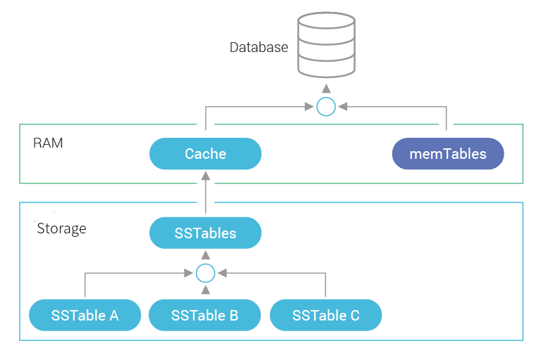
When the database is queried a node tries to locate the requested data in cache and memtables, both of which reside in RAM. If the data is in the cache – good, all that is needed is to combine the data from the cache with the data from memtable (if any) and a reply can be sent right away. But what if the cache has no data (and no indication that data is not present in permanent storage as well)? In this case, the bottom part of the diagram has to be invoked and storage has to be contacted.
The format the data is stored in is called an sstable. Depending on the configured compaction strategy, and on how recently queried data was written and on other factors, multiple sstables may have to be contacted to satisfy a request. Let’s take a closer look at the sstable format.
Very Brief Description Of the SSTable Format
Each sstable consist of multiple files. Here is a list of files for a hypothetical non-compressed sstable.
la-1-big-CRC.db
la-1-big-Data.db
la-1-big-Digest.sha1
la-1-big-Filter.db
la-1-big-Index.db
la-1-big-ScyllaDB.db
la-1-big-Statistics.db
la-1-big-Summary.db
la-1-big-TOC.txt
Most of those files (green ones) are very small and their content is kept in memory while the sstable is open. But there are two exceptions: Data and Index (as indicated in red). Let’s take a closer look at what those two contain.
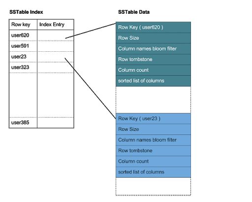
The Data file stores the actual data. It is sorted according to partition keys, which makes binary search possible. But searching for a specific key in a large file may require a lot of disk access, so to make the task more efficient there is another file, Index, that holds a sorted list of keys and offsets into the Data file where data for those keys can be found.
As one can see, each access to an sstable requires at least two reads from disk (it may be even more depending on the size of the data that has to be read and the place of the key in the index file).
Benchmarking ScyllaDB
Let’s look at how those maximum latencies can affect the behaviour of ScyllaDB. The benchmark was run on a cluster in the Google Compute Engine (GCE) with one NVMe disk. We have experienced that NVMe on GCE is somewhat slow, so in a way it helps to emphasis in-memory benefits. Below is a graph of 99th percentile for access to two different tables. One is a regular table on NVMe disk (red) and another is in memory (green).
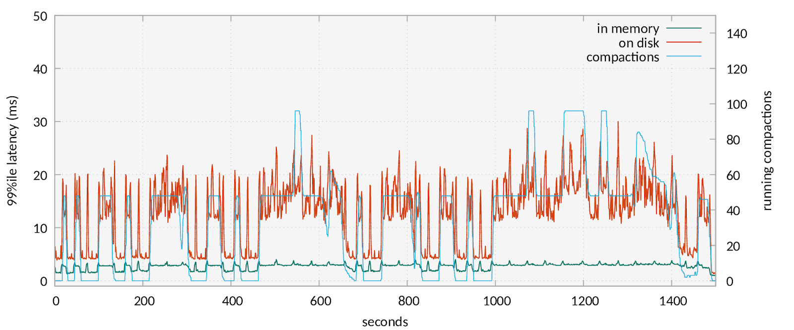
The 99th percentile latency for the on-disk table is much higher and has much more variation in it. There is another line in the graph (in blue) that plots the number of compaction running in the system. It can be seen that the blue graph matches the red one which means that 99th percentile latency of an on-disk table is affected greatly by the compaction process. High on-disk latencies here are a direct result of tail latencies that occurred because user read was queued after compaction read.
Having performance of 20ms for P99 isn’t much for ScyllaDB but in this case, a single not-so-fast NVMe disk was used. Adding more NVMes in raid0 setup will allow for more parallelism and will mitigate the negative effects of queuing, but doing so also increases the price of the setup and at some point will erase all the price benefits of using NVMe while not necessarily achieving the same performance as in-memory setup. In-memory setup allows you to get low and consistent latency at a reasonable price point.
Configuration
Two new configuration steps are needed to make use of the feature. First, one needs to specify how much memory should be left for in-memory sstable storage. It can be done by adding in_memory_storage_size_mb to scylla.yaml file or specifying --in-memory-storage-size-mb on a command line. After memory is reserved in-memory table can be created by executing:
CREATE TABLE ks.cf (
key blob PRIMARY KEY,
"C0" blob,
) WITH compression = {}
AND read_repair_chance = '0'
AND speculative_retry = 'ALWAYS'
AND in_memory = 'true'
AND compaction = {'class':'InMemoryCompactionStrategy'};
Note new in_memory property there that is set to true and new compaction strategy. Strictly speaking it is not required to use InMemoryCompactionStrategy with in-memory tables but this compaction strategy compacts much more aggressively to get rid of data duplication as fast as possible to save memory.
Note that mix of in-memory and regular tables is supported.
Conclusion
Despite what the vendors may say, real world storage devices can present high tail latencies in the face of competing requests, even for newer technology like NVMe. Workloads that cannot tolerate a jump in latencies under any circumstances can benefit greatly from the new ScyllaDB enterprise in-memory feature. If, on the other hand, a workload can cope with occasionally higher latency for a low number of requests it is beneficial to let ScyllaDB manage what data is held in memory with its usual caching mechanism and to use regular on-disk tables with fast NVMe storage.
Find out more about ScyllaDB Enterprise