Best Practices for Data Modeling

By Peter Corless

August 20, 2019

Update: For a deep dive into data modeling best practices, see the NoSQL Data Modeling Masterclass. It offers 3 hours of video instruction, free and on demand.

In our latest Summer Tech Talks series webinar ScyllaDB Field Engineer Juliana Oliveira guided virtual attendees through a series of best practices on data modeling for ScyllaDB. She split her talk into understanding three key areas:

How data modeling works in ScyllaDB
How data storage works and how data is compacted
How to find and work with (or around) large partitions

Juliana emphasized the criticality to mastering these fundamentals. “Because once we have the right conceptual model of how data is stored and distributed what follows gets natural.”

SQL vs. CQL

For those coming from a SQL background, Juliana first began by delineating the key differences between that well-known data model and the Cassandra Query Language (CQL) ScyllaDB uses.

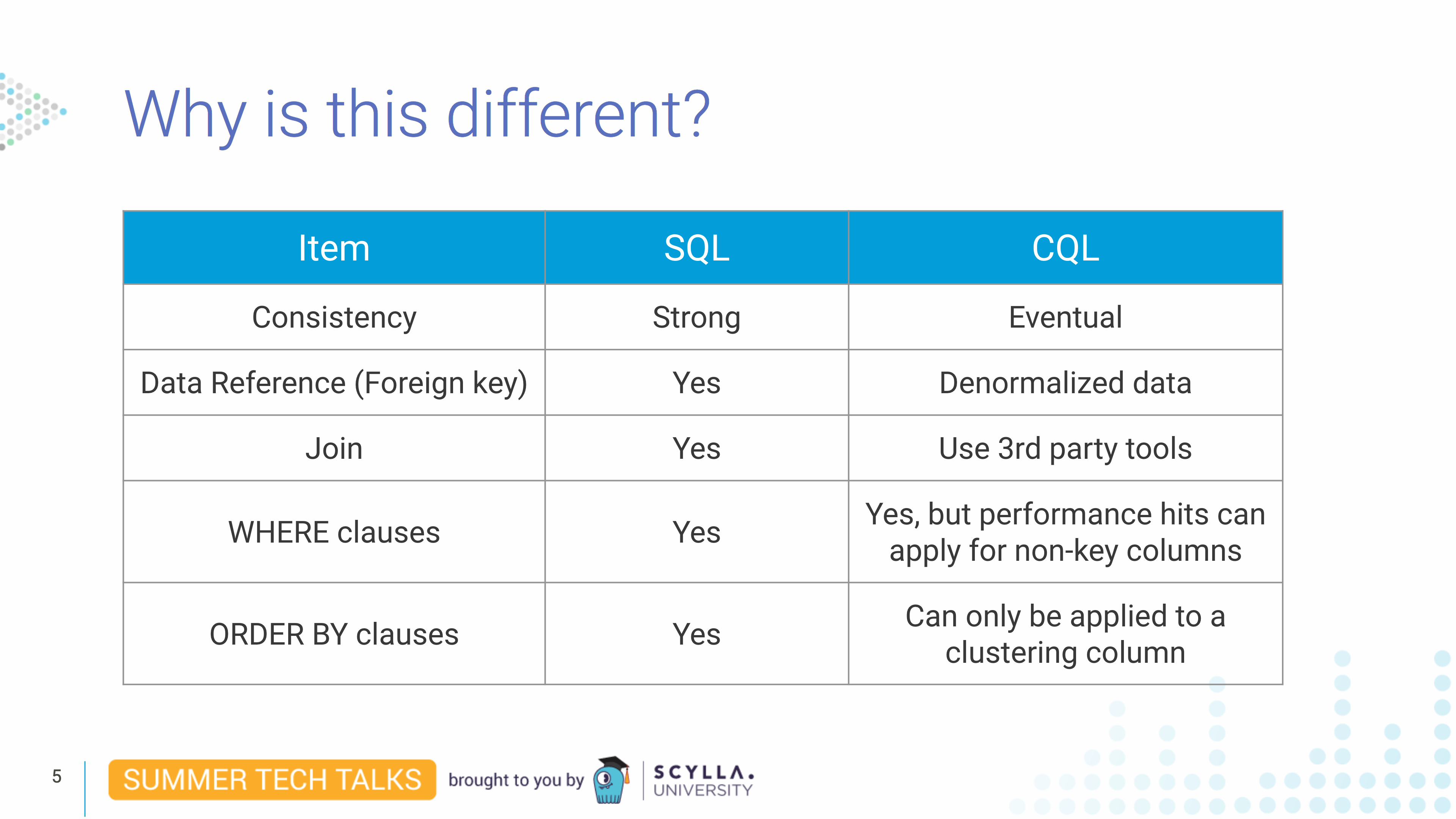
While there are similarities between the two query languages, Juliana noted “SQL data modeling cannot be perfectly applied to ScyllaDB.” You don’t have the same relational model to avoid data duplication. Instead, in ScyllaDB, all the data is denormalized. You also want to organize the data based on the queries you wish to execute. For example, you want to spread your data evenly across every node in the cluster so that every node holds roughly the same amount of data. Balancing should also be done to ensure you do not have “hot partitions” (frequently-accessed data) and data is evenly distributed across the nodes of the cluster. Therefore, determining your partition key is crucial.

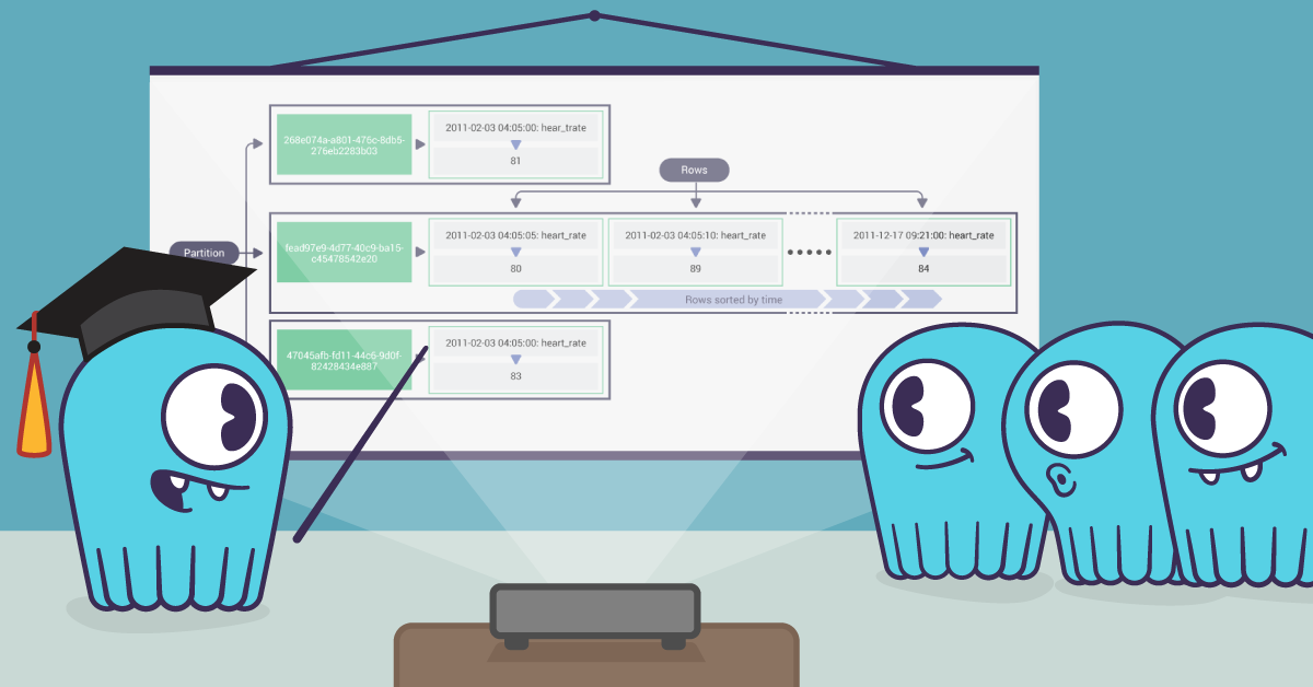
Partitions and Rows: A Veterinary Example

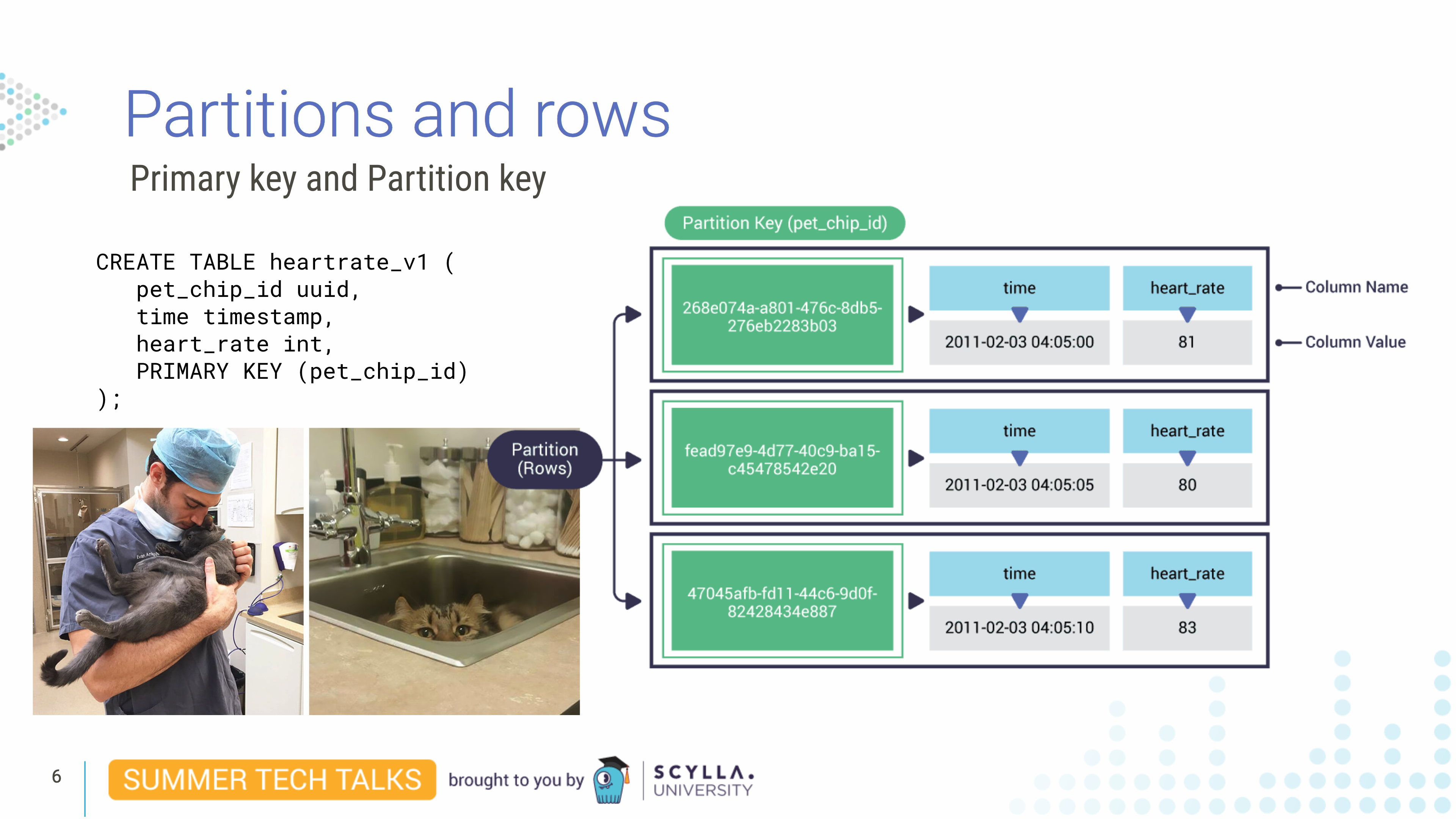
Imagine you work for a veterinary clinic. We create a table called heartrate_v1. In this table we have a pet_chip_id column, time column and a heart_rate column. We set the PRIMARY KEY to the pet_chip_id. The table is responsible for holding data for our pet patients. Imagine that we’re getting a new reading every five seconds. In this case, since pet_chip_id is our primary key, our unique identifier for rows in CQL, it is the unique identifier for a partition.

What is a partition?

A partition is a subset of the data on a node — a collection of sorted rows, identified by a unique primary key, or partition key. It is replicated across nodes.

In this case, we only have one column in the primary key field — the pet_chip_id. But since we are reading data every five seconds and the primary key must be unique, this is certainly not the ideal solution because if a reading comes in with that same pet_chip_id, it would write over the existing record.

What is a clustering key?

Now that we figured out that because of our data model we’re constantly overwriting our data, maybe we should add a new second column to the primary key. If we add time as a second column to the primary key field, this serves as a clustering key. What a clustering key does is sort each row physically inside the partition.

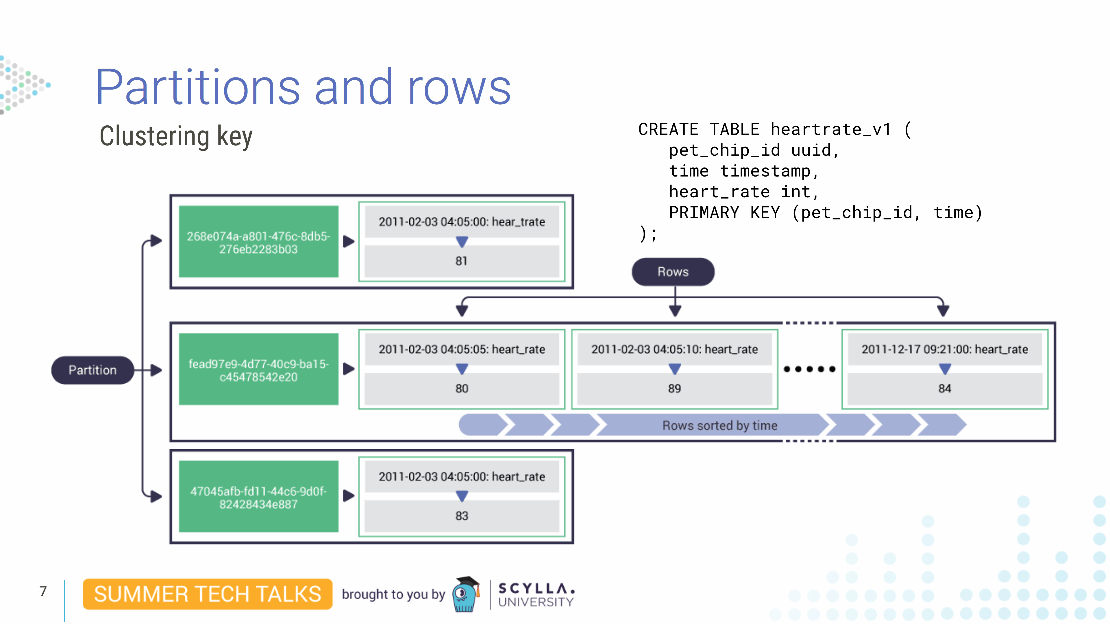
As we will see later, partition keys are hashed and distributed around the cluster. That means that queries always need to specify the partition key with an equality — since hashing will shuffle its natural sorting. But because the clustering key is not hashed the behavior is different.

When you write a query, you need to include the partition key but the clustering keys may be omitted, in which case the query acts on the entire partition, Also, because clustering keys are sorted inside the partition, you can also run queries with equalities and inequalities for the clustering keys.

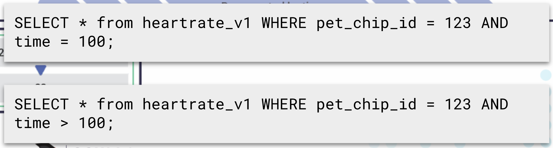
However, if you had two clustering keys, say, by heart_trate and time, you would sort by the clustering key order. First it would be sorted by time, and then by heart_rate. We cannot write a query specifying heart rate and not time, because data is physically by the clustering key order. So this query would fail because it doesn’t specify time; it only specifies heart_rate:

So knowing how a clustering key works, and knowing that we are writing heart_rate every five seconds it is easy to imagine a partition key growing quite large. Since pets can stay under monitoring for weeks we can have thousands of rows in the same partition. (For example, just one week of sampling a pet every five seconds would result in 120,960 rows in a single partition.) And having a partition this big could lead to performance problems, especially if you don’t know this is happening.

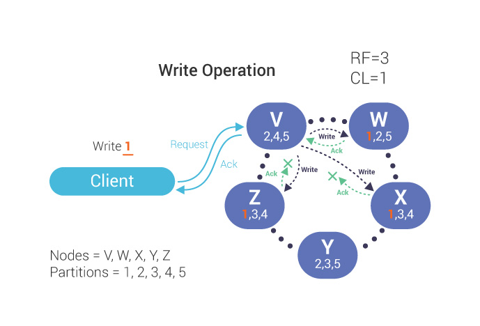
What happens to my partition key?

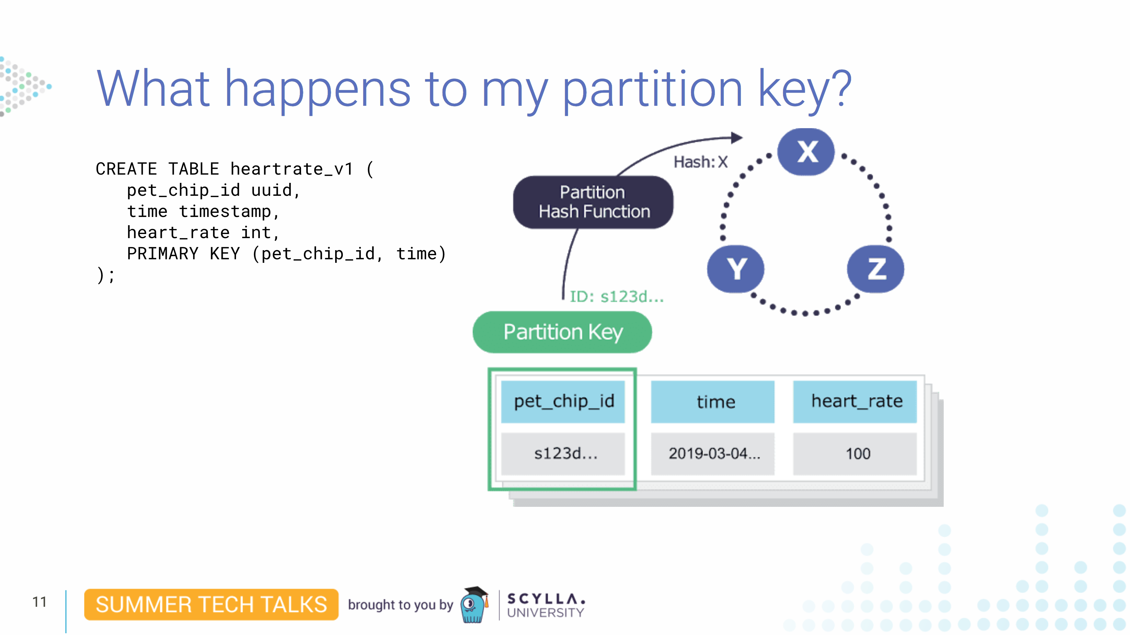
Where did it go? The partition key, which is pet_chip_id, will get hashed by our hash function — we use murmur3, the same as Cassandra — that generates a 64-bit hash. And then we’ll assign a partition key range for each node that will be responsible for storing keys.

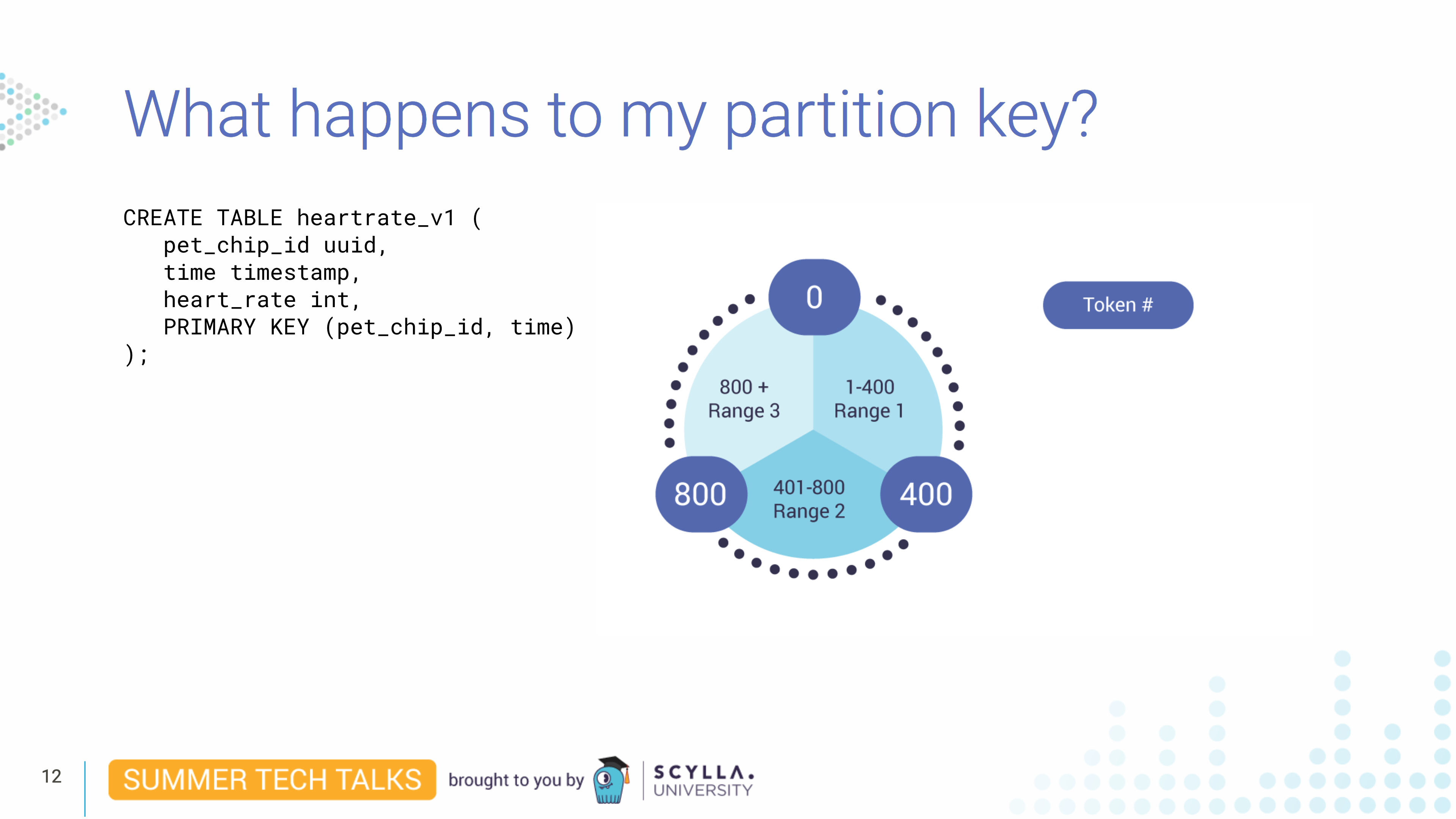
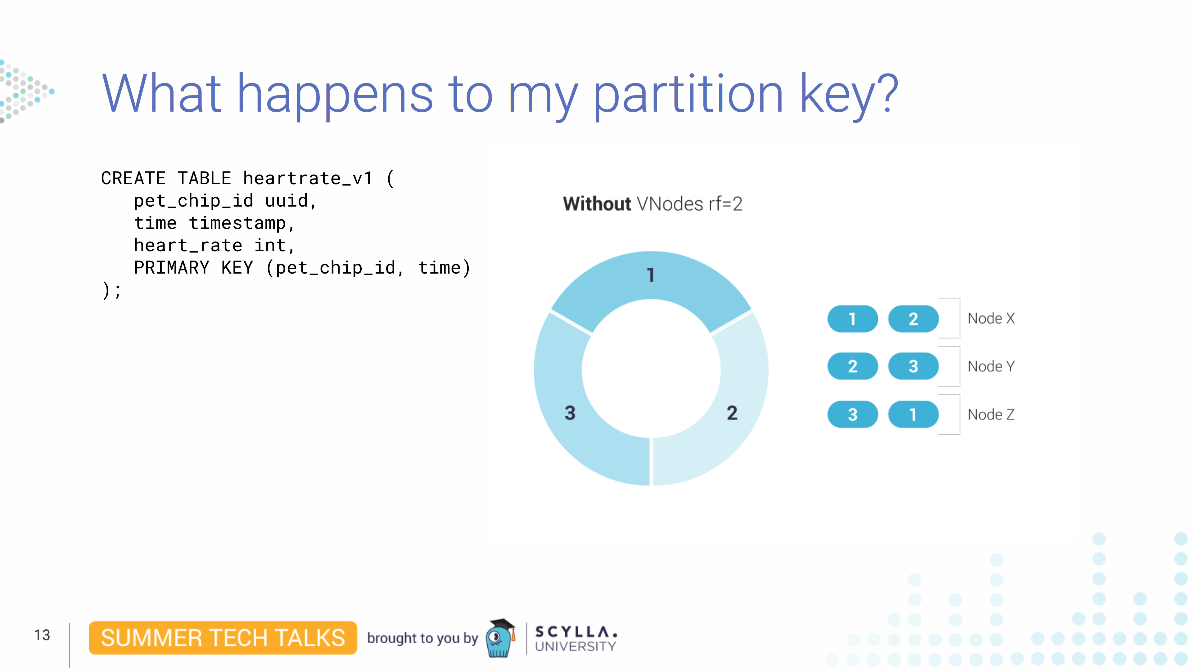
In this example you have a three-node cluster that is placing a token range from 0 to 1200. If you have a replication factor of 2, what will happen is each node holds two ranges. In reality what happens is that ScyllaDB splits data into vNodes. Without vNodes, and a replication factor of 2, the ring would look like this, where each node will be the primary for one partition key range, and will be the secondary for a second partition key range:

With vNodes, this is how ScyllaDB will split the data, where each physical node will be the primary replication for four ranges and the secondary replication for four others:

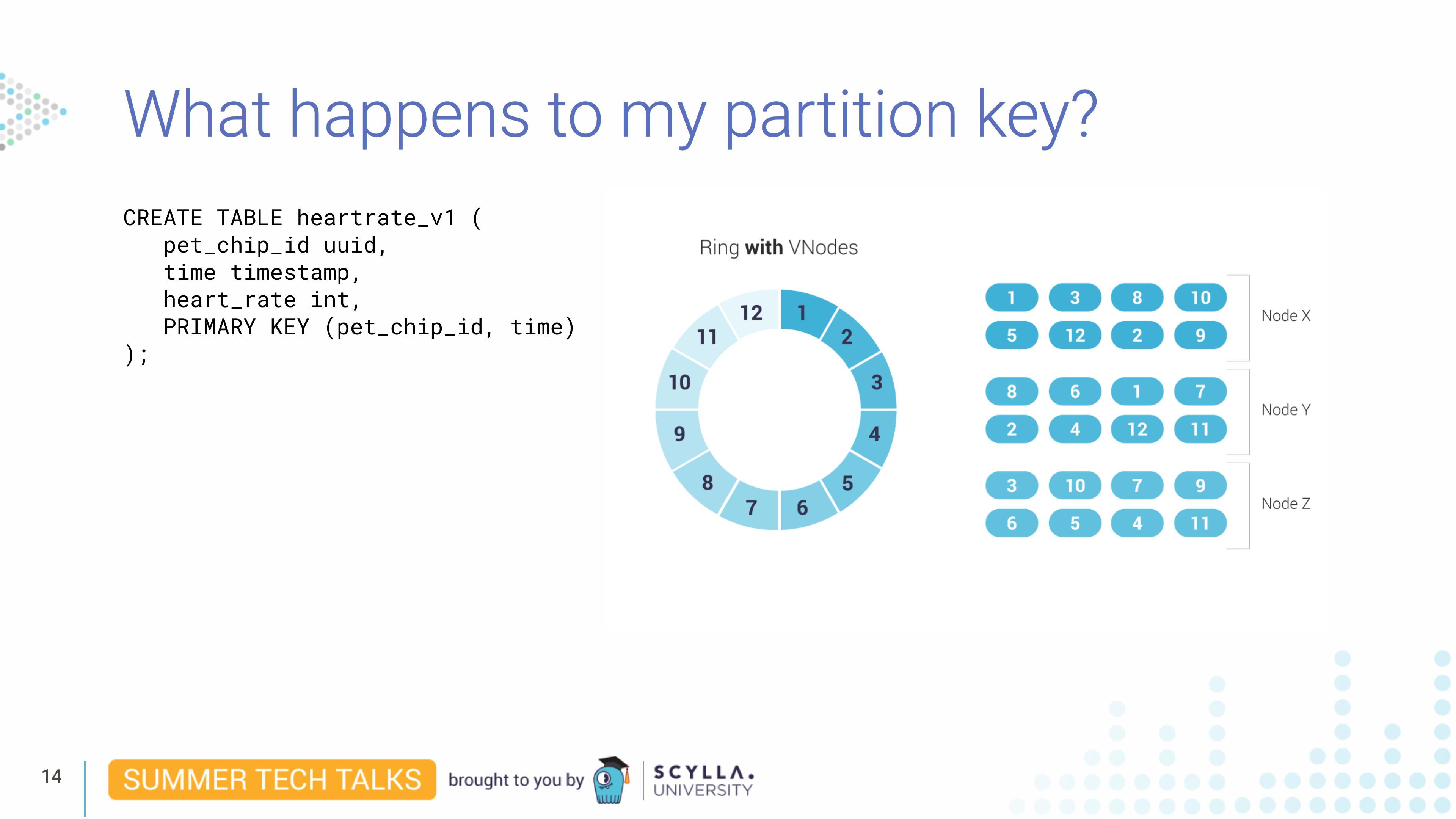
Having vNodes especially improves cluster rebuilding streaming times. Our partition key, a pet_chip_id, will reside in one of those vNode ranges (and its replicated copies). ScyllaDB knows where its is because of the hashing function.

Storage

Next Juliana turned to look at the underlying storage system in ScyllaDB, since this affects data modeling. To begin with, it is important to know that data is first written to an in-memory structure, the memtable. And, over time, a number of memtable changes will be flushed to persistent storage in an immutable (non-changing) file called an SSTable. So imagine in this first SSTable 1 we write some data that says “A = 1.”

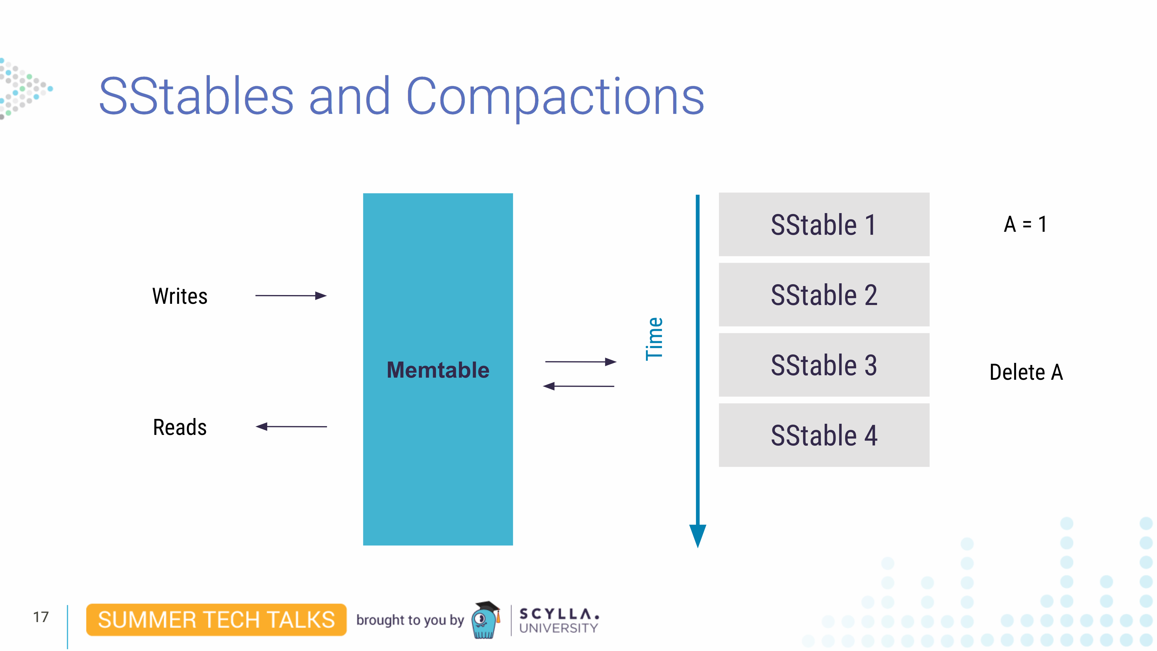
Over time, more data is flushed to additional SSTables. Imagine we eventually delete “A,” and in a memtable flush this update was written to SSTable 3. Knowing that an SSTable is immutable, what happens to it? We cannot delete “A” from our existing SSTables. So in this case, “A” will eventually be deleted in the next compaction.

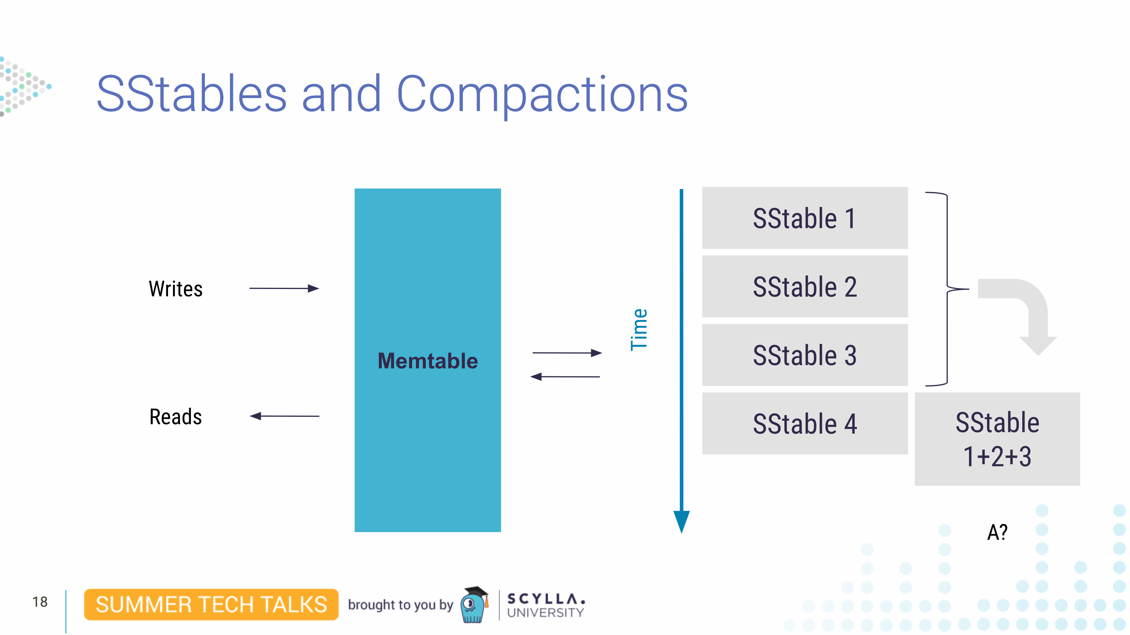
A compaction is an operation where a group of SSTables are read and their data combined to write a new SSTable containing only “live” (current) data. This is efficient because as SSTables are sorted we read only once and when data is compacted from multiple SSTables — 1+2+3 — they are checked for their most-updated values. So, for example the most updated value for “A” is “Delete it,” it gets deleted from the resulting SSTable 1+2+3 compaction. This is why when we delete data we won’t see it reflected on disk space until the next compaction.

There are different strategies, each associated with different algorithms of when and how to run compactions. Let’s list the main ones here:

By default, ScyllaDB uses size-tiered compaction strategy (STCS), which is very efficient. It compacts SSTables into similar-sized buckets so all SSTables have around the same size. But the downside is since we need to read before writing if your SSTables are too big it can take a lot of disk space. (This compaction strategy requires about 50% of your disk space free to write out large compactions. See also this blog.)
Time window compaction strategy (TWCS) uses size-tiered compaction as well; but with time window buckets. it is designed for use with time-series data.
Leveled compaction strategy (LCS) doesn’t require half of the disk space to be available, and separates the data by having multiple levels. This requires, however, more I/O on writes, so it is inefficient for write-heavy workloads.

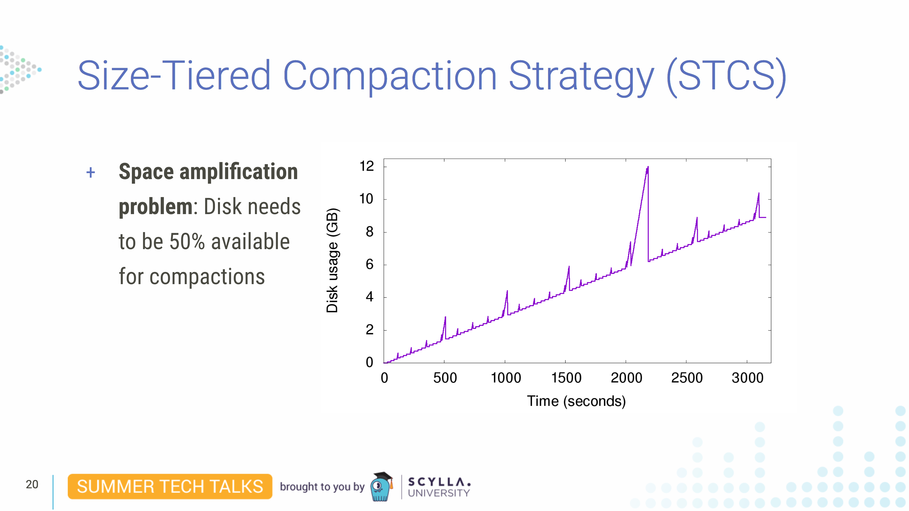
Size-tiered compaction strategy is the default used by ScyllaDB and it is triggered when the system has enough SSTables with similar sizes. As you can see in this graph it has disk usage spikes. They happen when ScyllaDB compacts all SSTables. For example, when we believe records are taking too much space and we want to get rid of them by running nodetool compact, which compacts all SSTables. So the input SSTables cannot be deleted until we finish writing the output SSTable. Right before the end of the compaction we have the data on disk twice, in the input SSTables and the (compacted) output SSTable. We temporarily need the disk space to be twice as large as the data available in the database. So for this compaction strategy to work we need for the disk to be half-full all the time.

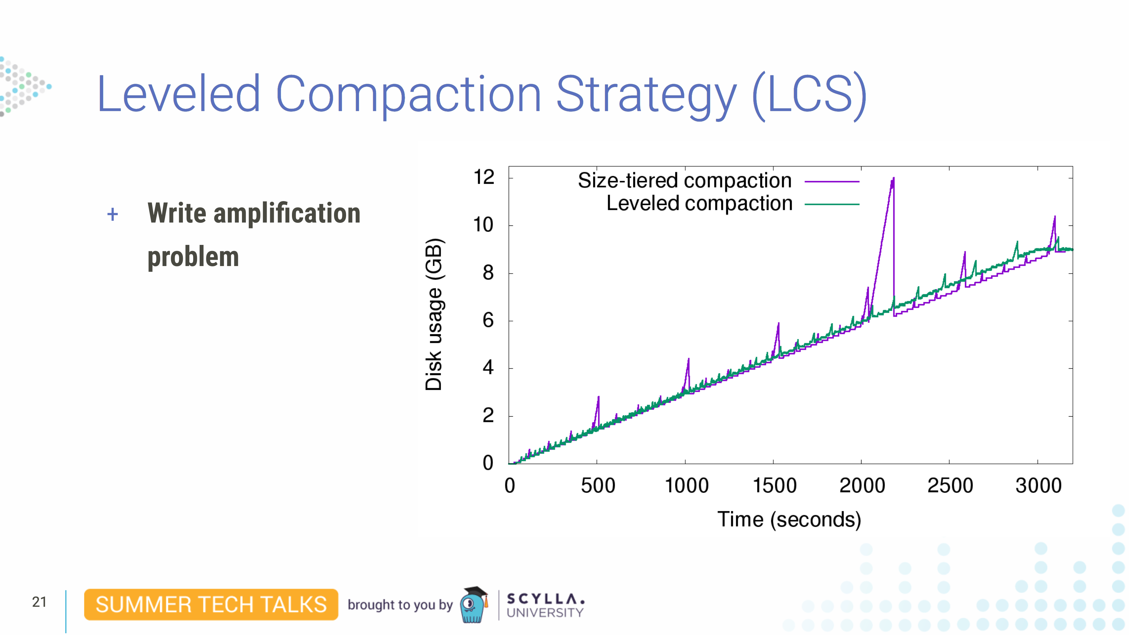
In this strategy, Leveled Compaction Strategy (LCS), evenly-sized SSTables are divided in levels. Each compaction generates a small SSTable which goes to the next level eventually. Since each small SSTable doesn’t have an overlapping key range they can be compacted in parallel. And also because they are small and never have to write a huge SSTable you don’t have the same space problem of size-tiered compactions.

The downside of the strategy is since we need to rewrite the same data every time an SSTable changes levels it can be I/O intensive.

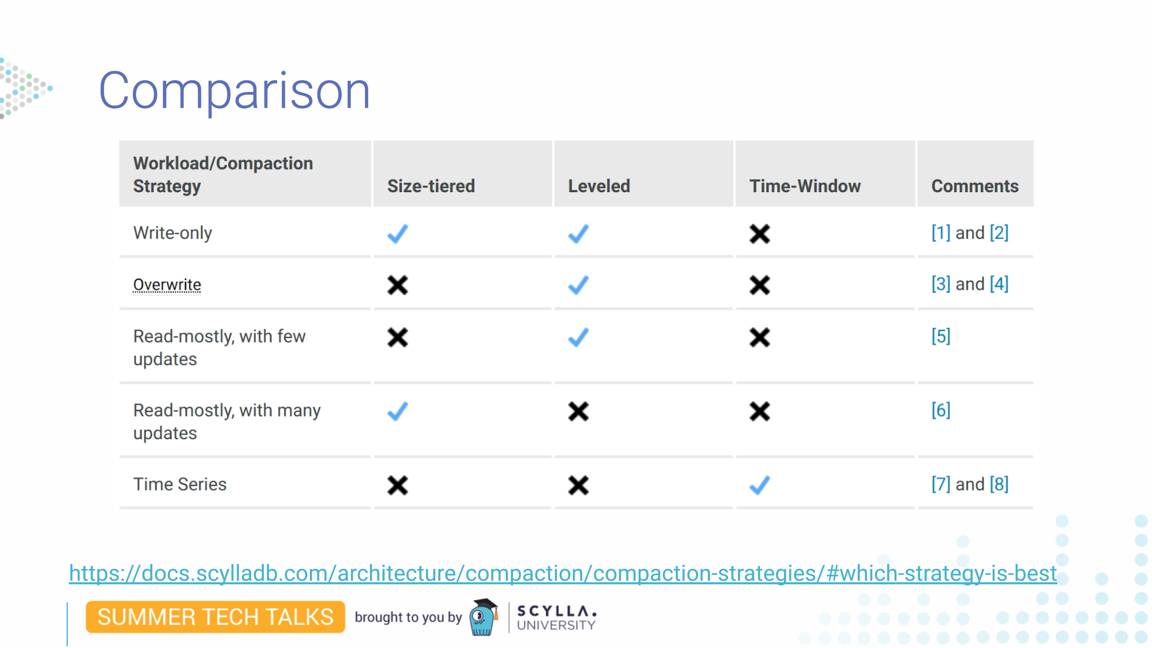
Here we can see that each has its advantages. Size-tiered and leveled work for write-only workloads, but one will take twice the disk space and the other will take twice the write operations. Leveled works best for overwrite data since it won’t keep all data as long as size-tiered. For many updates, leveled might be a problem since it also requires many writes.

There are many things to consider. If you are in any doubt which is the best strategy you should check our documentation.

Large Partitions and Hot Partitions

What are they? As we saw when talking about clustering keys we can have a huge number of values under a clustering key in the same partition. Leading to a monstrous number of rows in the partition. Such a partition is called a large partition and this is a problem because when you read it queries may be slower because ScyllaDB does not index the rows inside a partition and also because queries within a partition cannot be parallelized.

This can get worse. You can have a large partition problem combined with a hot partition problem. Which is when one of the partitions is particularly more-accessed than the others. This hot partition problem usually happens when data is badly distributed. For example, in the pet clinic we have one particular pet that is always sick. So we generate and we mark data for this pet.

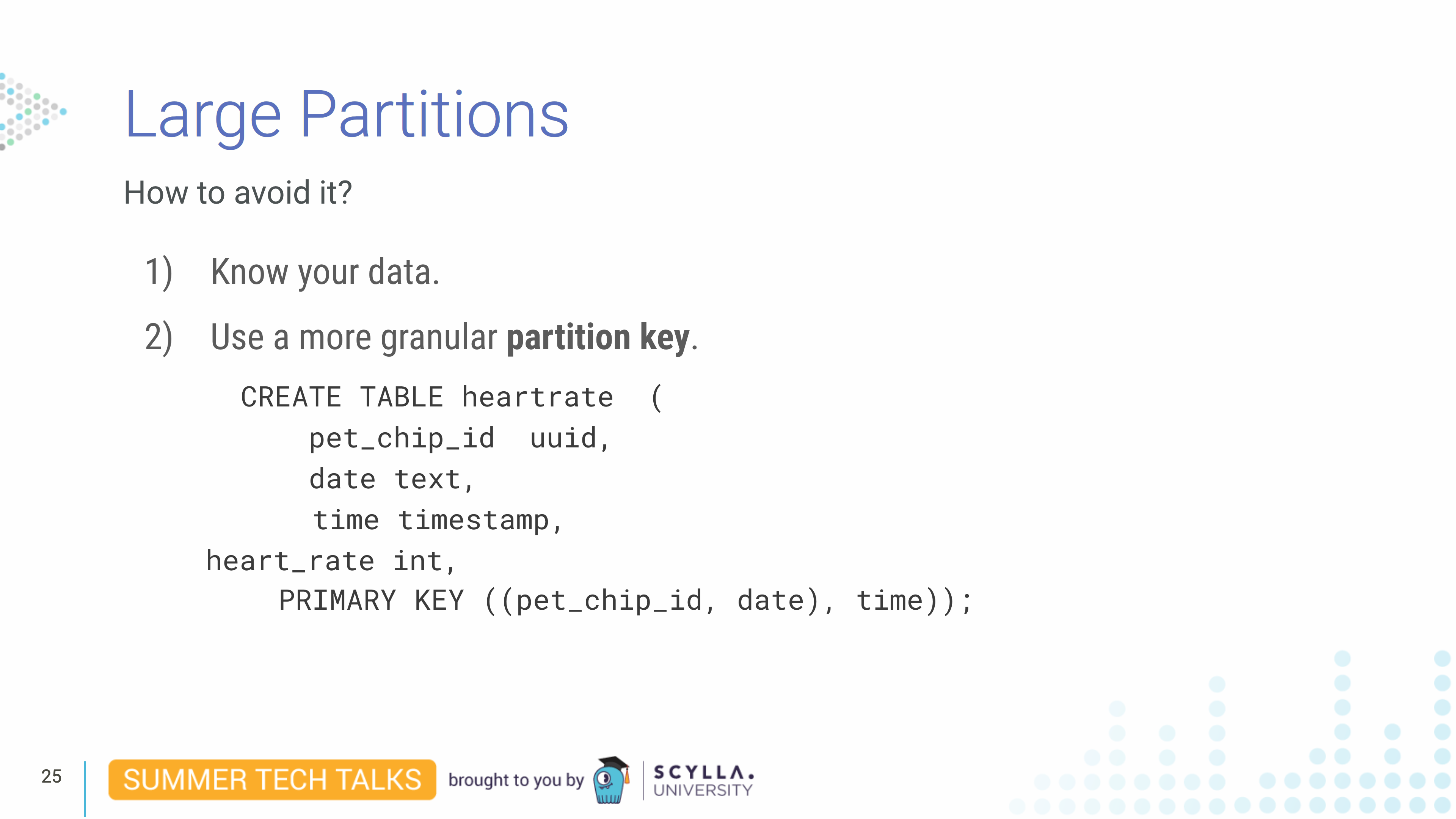
We have ways to avoid this kind of situation. First, you need to know your data and how it behaves. Second, it’s common to add granularity by adding more columns to the partition key. In this example we have a heart rate table and we added date to the primary key. So our partition is not only by pet_chip_id but also by date. This makes partitions smaller and easier to manage.

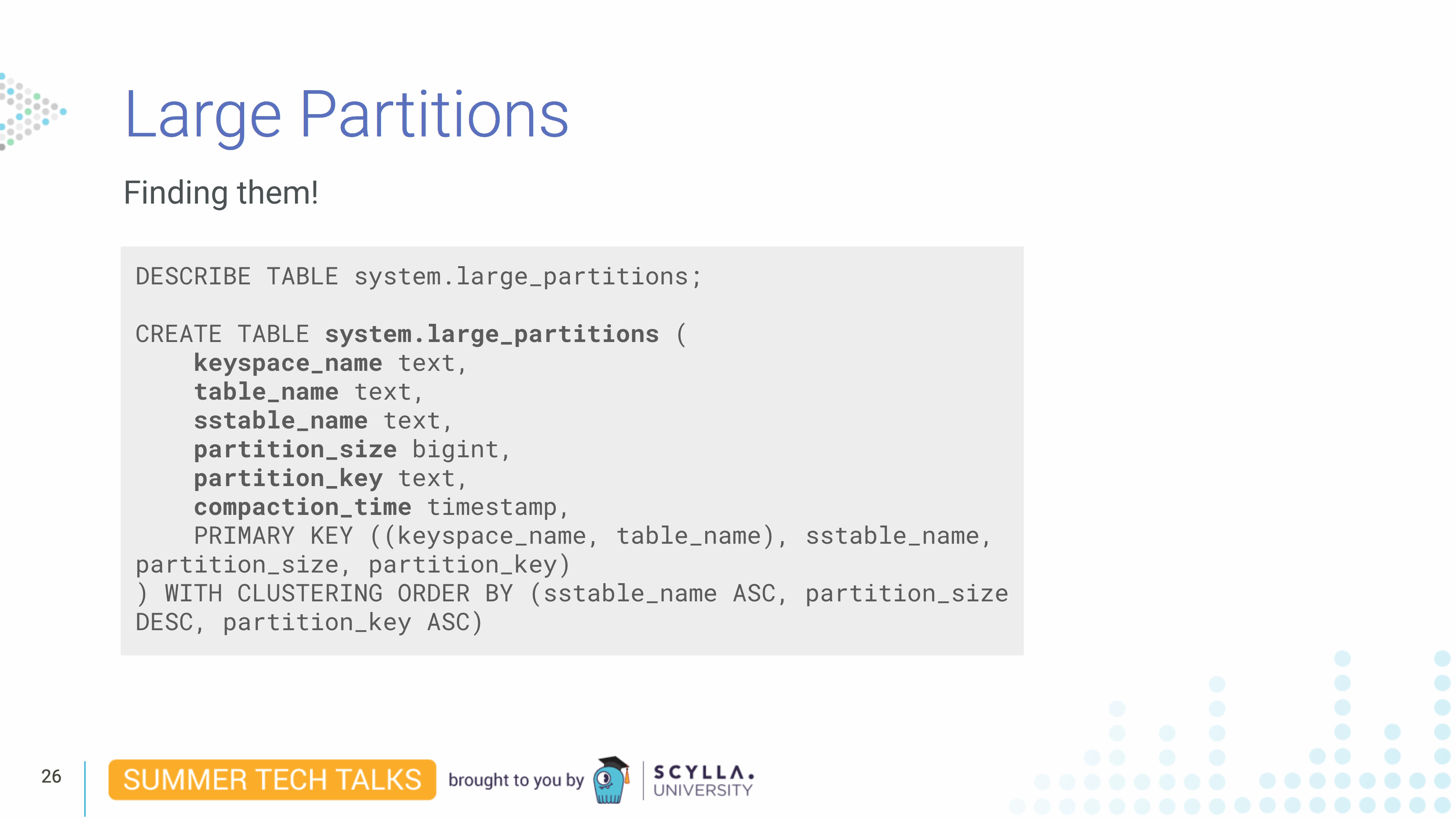
In order to track large partition we keep a system table called system.large_partitions. Every time a large partition is written to disk — which means, after it is flushed out of memtable — we add an entry to this table. It is possible to detect how many large partitions are generated over time in order to understand how your data behaves and improve on data distribution as needed. Note that this data will only be available after data is written to disk, not before.

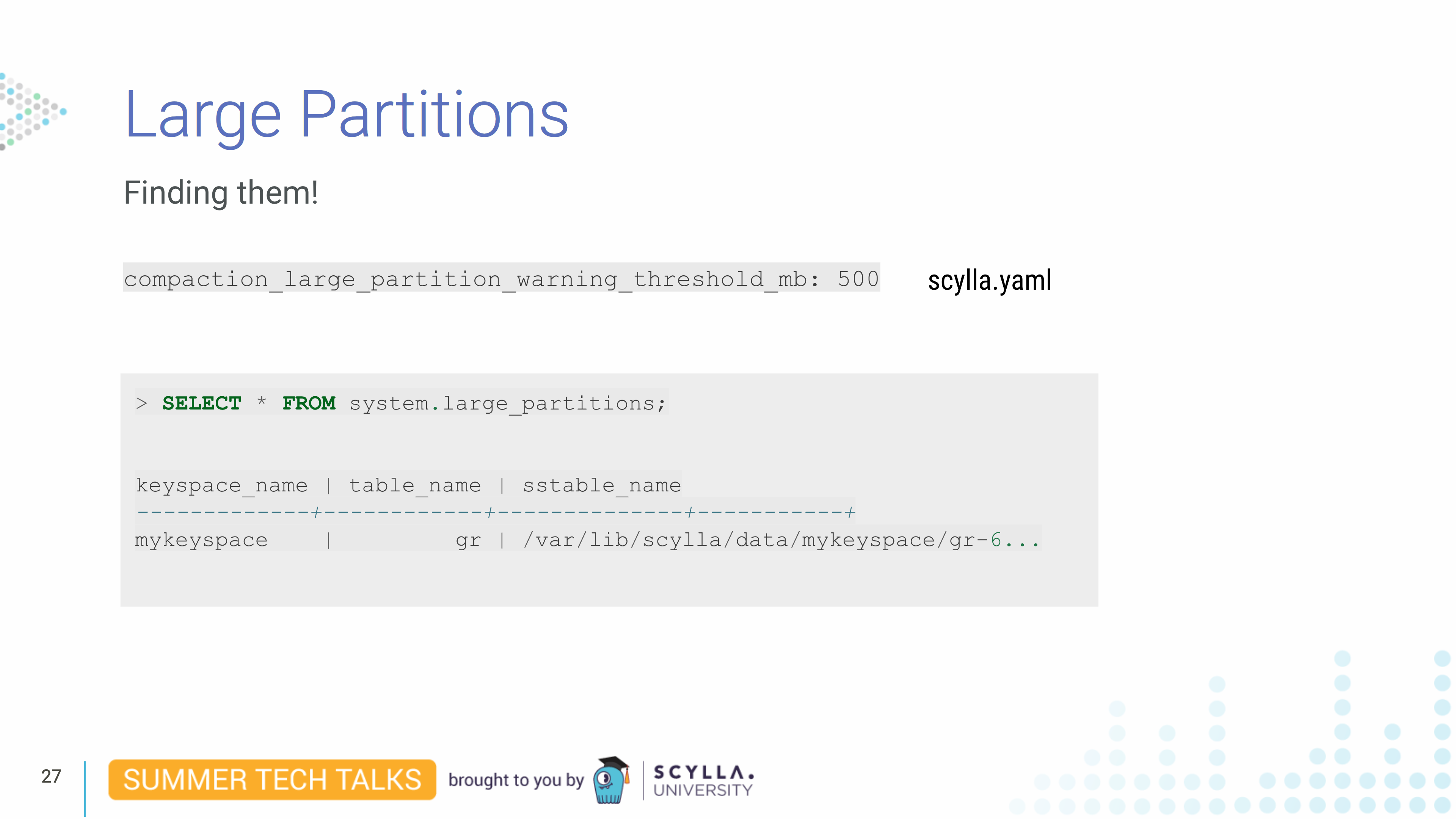
The large partition detection threshold can be set in the scylla.yaml file with the compaction_large_partion_warning_threshold_mb parameter, which defaults to 100 megabytes. You can use whatever you find relevant to your use case. Each partition bigger than this threshold is going to be reported in the large partitions table and in a written warning in the log so you can also set up alarms on your logging systems.