Note to readers: this blog entry uses JavaScript to render LaTeX equations, make sure it’s enabled.
Today’s databases commonly store terabytes to petabytes of data and handle hundreds of thousands to millions of client requests per second. A single server machine is not sufficient to handle such workloads. How do we make a database that doesn’t collapse under its own weight? How do we make a scalable, distributed database system?
But there’s more: modern databases are fault tolerant. Even if a piece of the system fails, the system still runs. How is that done? And how is this related to scalability? The answer to creating a scalable, fault-tolerant database system lies with the data partitioning and data replication within the architecture.
Partitions
In our quest to make a scalable database system we’ll first identify a logical unit of data which we’ll call a partition. Partitions shall be independent pieces that can be distributed across multiple machines.
Consider a key-value store. It is a type of database with a simple interface: to the user, it looks like a set of (key, value) pairs, e.g.:
| key | value |
| “k1” | “aaa” |
| “k2” | “bbb” |
| “k3” | “ccc” |
The store might support operations such as writing a value under a key, reading a value under a key or performing an atomic compare-and-set.
In such a store we can define a partition to simply be a (key, value) pair. Thus above, the pair \((“k1”, “aaa”)\) would be a partition, for example. I’m assuming that the different keys are not related, hence placing them far away from each other does not introduce certain subtle challenges (the next example explains what I have in mind).
On the other hand, consider a relational database. This type of database consists of relations (hence the name): sets of tuples of the form \((x_1, x_2, \dots, x_n)\), where \(x_1\) comes from some set \(X_1\), \(x_2\) comes from some set \(X_2\), and so on. For example, suppose \(X_1\) is the set of integers, \(X_2\) is the set of words over the English alphabet, and \(X_3\) is the set of real numbers; an example relation over \(X_1\), \(X_2\) and \(X_3\) would be
| X1 | X2 | X3 |
| 0 | “aba” | 1.5 |
| 42 | “universe” | π |
| 1 | “cdc” | -1/3 |
The sets \(X_i\) are usually called columns, the tuples — rows, and the relations — tables. In fact, a key-value store can be thought of as a special case of a relational database with two columns and a particular constraint on the set of pairs.
Some columns of a table in a relational database may serve a special purpose. For example, in Cassandra and ScyllaDB, clustering columns are used to sort the rows. Therefore rows are not independent, unlike the (key, value) pairs from the previous example.
Maintaining a global order on rows would make it very hard to scale out the database. Thus, in Cassandra and ScyllaDB, rows are grouped into partitions based on another set of columns, the partitioning columns. Each table in these databases must have at least one partitioning column. A partition in such a table is then a set of rows which have the same values in these columns; these values together form the partition key of the row (Cassandra partition key / ScyllaDB partition key). Order based on clustering columns is maintained within each partition, but not across partitions.
Suppose our table has a partitioning column pk and a clustering column ck. Each column has the integer type. Here’s what the user might see after querying it:
| pk | ck |
| 0 | 2 |
| 0 | 3 |
| 2 | 0 |
| 2 | 1 |
| 1 | 5 |
In this example there are 3 partitions: \(\{(0, 2), (0, 3)\}\), \(\{(2, 0), (2, 1)\}\), and \(\{(1, 5)\}\). Note that within each partition the table appears sorted according to the clustering column, but there is no global order across the partitions.
For a general relational database we can assume the same strategy: a subset of columns in a table is identified as partitioning columns, and the partitions are sets of rows with common values under these columns. This will lead us to what’s usually called horizontal partitioning; the name is probably related to the way tables are usually depicted.
The important thing is that each partition has a way of uniquely identifying it, i.e. it has a key; for relational databases, the key is the tuple of values under partitioning columns for any row inside the partition (the choice of row does not matter by definition). For key-value stores where partitions are key-value pairs, the partition’s key is simply… the key.
In the above example, the key of partition \(\{(0, 2), (0, 3)\}\) is \(0\), for \(\{(2, 0), (2, 1)\}\) it’s \(2\), and for \(\{(1, 5)\}\) it’s \(1\).
How To Design a Fault-Tolerant Database System
We’ve identified the partitions of our database. Now what?
Here’s how a non-distributed store looks:
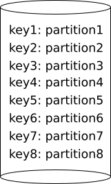
There is one node which stores all the partitions. This works fine as long as:
- you make regular backups so that you don’t lose your data in case your node burns down and you don’t care if you lose the most recently made writes,
- all the partitions fit in a single node,
- the node keeps up with handling all client requests.
And now we’re going to cut our data into pieces.
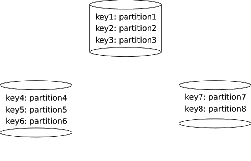
This cutting is called sharding. The parts that we obtained are typically called shards in the database world. In this example we have 3 shards: one with keys \(\{key1, key2, key3\}\), one with \(\{key4, key5, key6\}\), and one with \(\{key7, key8\}\). Sometimes shards are also called ranges or tablets.
ScyllaDB also uses “shards” to refer to CPU cores, which is a term that comes from the Seastar framework ScyllaDB is built on top of. This concept of shard is not related in any way to our current discussion.
Now we have a sharded database; for now we’ve put each shard on a single node. Within each shard a number of partitions is kept.
Sharding solves two issues:
- Partitions occupy space, but now they are distributed among a set of nodes. If our DB grows and more partitions appear we can just add more nodes. This is a valid strategy as long as the partitions themselves don’t grow too big: in ScyllaDB we call this “the large partition problem” and it’s usually solved by better data modeling. You can read about how ScyllaDB handles large partitions.
- A node doesn’t need to handle all client requests: they are distributed according to the partitions that the clients want to access. This works as long as there is no partition that is everyone’s favorite: in ScyllaDB we call this “the hot partition problem” and as in the case of large partitions, it’s usually solved by better data modeling. ScyllaDB also collects statistics about the hottest partitions which can be investigated by the nodetool toppartitions command.
Our database now has the ability to scale out nicely if we take care to distribute data uniformly across partitions. It also provides some degree of fault tolerance: if one of the nodes burn down, we only lose that one shard, not all of them. But that’s not enough, as every shard may contain important data.
The solution is data replication: let’s keep each shard on a subset of nodes!
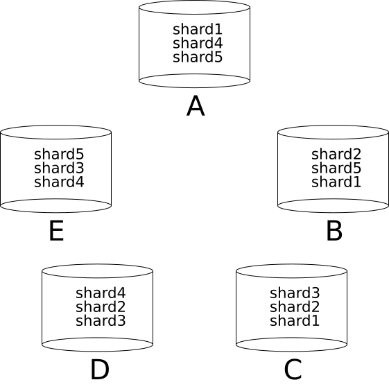
We probably don’t want to keep each shard on every node; that would undo our previous scalability accomplishment (but it may be a valid strategy for some tables). We keep them on a number of nodes large enough to achieve a high degree of fault tolerance. The location of each copy also matters; we may want to put each shard on at least two nodes which reside in different geographical locations.
For shard \(S\), the set of nodes to which this shard is replicated will be called the replica set of \(S\). In the example above, the replica of shard \(shard5\) is \(\{A, B, E\}\).
Partitioning schemes and data replication strategies
Each partition in our store is contained in a single shard, and each shard is replicated to a set of nodes. I will use the phrase partitioning scheme to denote the method of assigning partitions to shards, and replication strategy to denote the method of assigning shards to their replica sets.
Formally, let \(\mathcal K\) be the set of partition keys (recall that each key uniquely identifies a partition), \(\mathcal S\) be the set of shards, and \(\mathcal N\) be the set of nodes. There are two functions:
- \(\mathcal P: \mathcal K \rightarrow \mathcal S\), the partitioning scheme,
- \(\mathcal R: \mathcal S \rightarrow \mathbb P(\mathcal N)\), the replication strategy.
For a set \(X\), the symbol \(\mathbb P(X)\) denotes the power set of \(X\), i.e. the set of all subsets of \(X\).
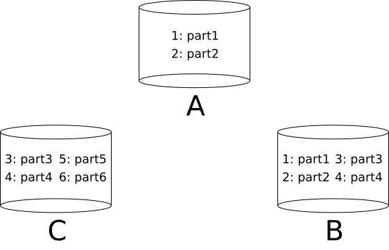
For example, suppose that \(\mathcal K = \{1, 2, 3, 4, 5, 6\}\), \(\mathcal S = \{s_1, s_2, s_3\}\), and \(\mathcal N = \{A, B, C\}\). One partitioning scheme could be:
\[ \mathcal P = \{ \langle 1, s_1 \rangle, \langle 2, s_2 \rangle, \langle 3, s_3 \rangle, \langle 4, s_2 \rangle, \langle 5, s_3 \rangle, \langle 6, s_6 \rangle \} \].
The notation \(f = \{\langle x_1, y_1 \rangle, \langle x_2, y_2 \rangle, \dots\}\) denotes a function \(f\) such that \(f(x_1) = y_1\), \(f(x_2) = y_2\), and so on.
One replication strategy could be:
\[ \mathcal R = \{ \langle s_1, \{A, B\} \rangle, \langle s_2, \{B, C\} \rangle, \langle s_3, \{C\} \rangle \} \].
To calculate where each key is, we simply compose the functions: \(\mathcal R \circ \mathcal P\). For example:
\[ (\mathcal R \circ \mathcal P)(3) = \mathcal R(\mathcal P(3)) = \mathcal R(s_2) = \{B, C\} \].
The end result for this partitioning scheme and replication strategy is illustrated below.
Sometimes the replication strategy returns not a set of nodes, but an (ordered) list. The first node in this list for a given shard usually has a special meaning and is called a primary replica of this shard, and the others are called secondary replicas.
We could argue that the notion of “partitioning scheme” is redundant: why not simply map each partition to a separate shard (i.e. each shard would consist of exactly one partition)? We could then drop this notion altogether and have replication strategies operate directly on partitions.
To this complaint I would answer that separating these two concepts is simply a good “engineering practice” and makes it easier to think about the problem. There are some important practical considerations:
- The partitioning scheme should be fast to calculate. Therefore it should only look at the partition key and not, for example, iterate over the entire set of existing partitions. That last thing may even be impossible since the set of partitions may be of unbounded size.
- If the partitioning scheme maps partition keys to a small, maintainable number of shards (say a couple thousands of them), we can afford the replication strategy to be a bit more complex:
- It can look at the entire set of shards when deciding where to replicate a shard.
- It can make complex decisions based on the geographical location of nodes.
- Due to the small number of shards we can easily cache its results.
Consistent hashing
A partitioning scheme is a method of grouping partitions together into shards; a replication strategy decides where the shards are stored. But how do we choose these two functions? If we consider all variables, the task turns out to be highly non-trivial; to make our lives simpler let’s make the following assumptions (it’s just the beginning of a longer list, unfortunately):
- Our database nodes have the same storage capacity.
- Our database nodes have the same computational power (both in terms of CPU and I/O).
From the top of my head I can list the following goals that we would like to achieve given these assumptions:
- Storage should be uniformly distributed across nodes.
- Client requests should be uniformly distributed across nodes.
It will be convenient to make some further assumptions:
- There are many partitions (like a lot). With large data sets and some good data modeling the number of partitions may count in millions, if not billions.
- The sizes of the large partitions are still small compared to the entire data set.
- Similarly, the numbers of requests to the most popular partitions are still small compared to the total number of requests.
- The distribution of workload across partitions is static.
One “obviously” desirable property of a partitioning scheme that comes to mind is to have it group partitions into shards of roughly equal size (in terms of storage and popularity of the contained partitions). That’s not strictly necessary, however: if the number of shards themselves is big enough, we can afford to have them a bit imbalanced. The replication strategy can then place some “smaller” shards together with some “bigger” shards on common replica sets, thus achieving the balancing of partitions across nodes. In other words, the responsibility of load balancing can be shifted between the partitioning scheme and the replication strategy.
Since we assumed that workload distribution is static, we can afford to have our two functions statically chosen (and not, say, change dynamically during normal database operation). However, there is still the problem of adding and removing nodes, which forces at least the replication strategy function to adjust (since its range \(\mc N\) changes); with that in mind let’s state another condition:
- if a new node is added, it should be easy to move the data; the moving process should not overload a single node but distribute the strain across multiple nodes.
A similar condition could be stated for the problem of removing a node.
Without further ado, let us introduce a simple partitioning scheme that uses a technique called consistent hashing. Consider a circle.
Let \(C\) denote the set of points on the circle. We start by choosing a small (finite) subset of points on the circle \(T \subseteq C\):
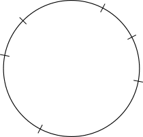
The elements of \(T\) are called tokens.
Now define a function \(first: C \rightarrow T\) which, given a point on the circle, returns the first token “to the right” of this point (imagine you start walking the circle from the point in the clockwise direction, stopping at the first token). E.g.:
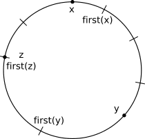
As the example shows for the point \(z\), if \(p \in T\), then \(first(p) = p\).
Now suppose that we have a function \(hash: \mathcal K \rightarrow C\) that given a partition key returns a point on the circle. Let’s assume that the function distributes the hashes uniformly across the circle. Our partitioning scheme is defined as follows:
\[ \mathcal P(k) = first(hash(k)). \]
Thus the range of \(\mathcal P\) is the set of tokens, \(T\); in other words, tokens are the shards of this partitioning scheme.
This scheme has a nice property which will turn out to be useful for us soon. Suppose that we randomly sample \(l\) tokens uniformly from the circle; then, on average, the portion of the circle that is mapped to any given token is \(1/l\). Thus, on average, the portion of the circle that is mapped to any \(m\) of these \(l\) tokens is \(m/l\). If the numbers \(l\) and \(m\) are large enough, we can expect the portion of the circle mapped to any \(m\) tokens to be pretty close to this average.
But how close? Let’s look at an example. Suppose we sample \(l = 1000\) tokens from the circle and look at the first \(m = 250\). What portion is mapped to these 250 tokens? “On average” it should be \(1/4\). I have repeated this experiment 10000 times and obtained the following results:
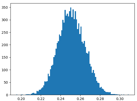
This shows that we can be almost certain that the portion of the circle mapped to our \(250\) out of \(1000\) randomly chosen tokens is between \(1/5\) and \(1/3\).
Now let’s define a simple replication strategy based on the circle of tokens. Suppose that we have chosen \(l\) tokens equal to some multiple \(m\) of the number of our nodes; say we have \(N\) nodes and we’ve chosen \(m \cdot N\) tokens. To each token we assign one of the nodes, called its owner, such that each node owns \(m\) tokens. Formally, we define a function \(owner: T \rightarrow \mathcal N\), with the property that the sets \(owner^{-1}(n)\) for \(n \in \mathcal N\) have size \(m\). Recall that the tokens are the shards in our partitioning scheme; we can define a replication strategy simply as follows:
\[ \mathcal R(t) = owner(t). \]
Now if the tokens were chosen randomly with uniform distribution, then:
- each node owns tokens that together are assigned on average \(1/N\) of the circle, where \(N\) is the number of nodes; if the multiple \(m\) is large enough (a couple hundreds will do), each portion is very close to that average,
- by our previous assumption, the hashes of partition keys are uniformly distributed around the circle,
- therefore each node replicates roughly \(1/N\) of all partitions.
Some nodes may get large/hot partitions assigned, but hopefully the hash function doesn’t decide to put all large/hot partitions in one place (it probably won’t since it uses only the key, it doesn’t care about the size/popularity of a partition), so each node receives a similar portion of their share of the problematic partitions. Even if one node is unlucky and gets a bit more of these, our assumptions say that they won’t make a significant difference (compared to the total workload generated by “common” partitions).
Furthermore, suppose we add another node and assign it additional \(m\) randomly chosen tokens, so we end up with \(m \cdot (N+1)\) tokens in total. Since randomly choosing \(m \cdot N\) tokens followed by randomly choosing additional \(m\) tokens is the same as randomly choosing \(m \cdot (N + 1)\) tokens in the first place (assuming the tokens are chosen independently), we now expect each of the \(N + 1\) nodes to replicate roughly \(1 / (N+1)\) of all partitions. Finally, convince yourself that during the process the new node stole from each existing node roughly \(1 / (N+1)\) of data owned by that node.
This replication strategy assigns only one replica to each shard, so it’s not very useful in practice (unless you don’t care about losing data), but it serves as an example for showing how the circle of randomly chosen tokens helps us distribute workload uniformly across nodes. In a follow up to this post we will look at some more complex replication strategies based on the circle of tokens. By the way, this scheme is used by both ScyllaDB and Cassandra (Cassandra sharding and replication); look for the phrase token ring.
At ScyllaDB we’re used to speaking about token ranges, also called vnodes: the intervals on the ring between two tokens with no token in between. There is a one-to-one correspondence between tokens and vnodes: the function that maps a token to the vnode whose right boundary is that token and left boundary is the token immediately preceding it on the ring. Vnodes are closed from the right side (i.e. they include the right boundary) and opened from the left side. The partitioning scheme can be thought of as mapping each partition key to the vnode which contains the key’s hash in between its boundaries.
One more thing: we’ve made an assumption that there exists a hash function \(hash: \mathcal K \rightarrow C\) mapping partition keys uniformly onto the circle. In practice, any “good enough” hash function will do (it doesn’t have to be a cryptographic hash). ScyllaDB represents the circle of tokens simply using the set of 64-bit integers (with some integers reserved due to implementation quirks) and uses the murmur hash function.
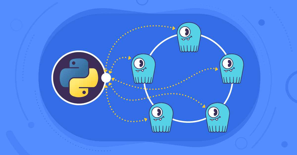
Putting Data Partitioning and Replication Into Practice
Now that you understand better how partitions and replication work in ScyllaDB, you can see how this was applied to the practical use of making a shard-aware driver in Python. A shard-aware driver needs to understand exactly which shard data is replicated on, to ensure one of the replicas is used as the coordinator node for a transaction. Part 1 takes the above and shows how ScyllaDB and Cassandra drivers work similarly, yet differ because of shard-awareness, and Part 2 shows how to implement a faster-performing shard-aware Python driver.