

Even a small, compact setup achieved up to 12,840 QPS at k=10 with a serial P99 latency of 5.5 ms
Our 1-billion-vector benchmark demonstrated that ScyllaDB Vector Search can sustain 252,000 QPS with 2 ms P99 latency across a large-scale deployment. But not every workload starts at a billion vectors. Many production use cases (e.g., product catalogs, knowledge bases for RAG, and semantic caches) live comfortably in the 10–100 million range.
This post presents a smaller benchmark: a 10-million-vector dataset of 768-dimensional Cohere embeddings on a compact five-node cluster. It used three modest storage nodes and two memory-optimized search nodes, all running on AWS Graviton. We explore four index configurations that span the recall-throughput spectrum, from near-perfect recall to maximum throughput. The results show that even this small setup can deliver up to 12,840 QPS at k=10 with a serial P99 latency of 5.5 ms — without any quantization.
Architecture at a Glance
First, some background. ScyllaDB Vector Search separates storage and indexing responsibilities while keeping the system unified from the user’s perspective. The ScyllaDB storage nodes hold both the structured attributes and the vector embeddings in the same distributed table.
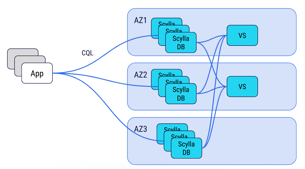
Meanwhile, a dedicated Vector Store service — implemented in Rust and powered by the USearch engine — consumes updates from ScyllaDB via CDC and builds approximate nearest neighbor (ANN) indexes in memory. Queries are issued through standard CQL:
SELECT … ORDER BY vector_column ANN OF ? LIMIT k;
The queries are internally routed to the Vector Store service, which performs the HNSW similarity search and returns the candidate rows. This design allows each layer to scale independently, optimizing for its own workload characteristics and eliminating resource interference. For a detailed architectural deep-dive, see the 1-billion-vector benchmark and the technical blog Building a Low-Latency Vector Search Engine for ScyllaDB.
Benchmark Setup
Here’s a look at the dataset and hardware used for the benchmark.
Dataset
| Property | Value |
| Vectors | 10,000,000 |
| Dimensions | 768 |
| Embedding model | Cohere |
| Similarity function | COSINE |
| Quantization | None (f32) |
Hardware
| Role | Instance | vCPUs | RAM | Count |
| Storage nodes | i8g.large | 2 | 16 GB | 3 |
| Search nodes | r7g.2xlarge | 8 | 64 GB | 2 |
With 768-dimensional f32 vectors and M values up to 64, the in-memory index size can be estimated as:
Memory ≈ N × (D × 4 + M × 16) × 1.2
For the largest configuration (M=64): 10M × (768 × 4 + 64 × 16) × 1.2 ≈ 49 GB, which fits comfortably in the 64 GB of a single r7g.2xlarge search node. No quantization is needed at this scale.
Experiments
We tested four HNSW index configurations, progressively lowering graph connectivity (M) and search effort (ef_search) to shift the balance from recall toward throughput.
| Experiment | M | ef_construction | ef_search | k tested |
| #1 (high quality) | 64 | 384 | 192 | 100, 10 |
| #2 (balanced) | 32 | 256 | 128 | 100, 10 |
| #3 (high throughput) | 24 | 256 | 64 | 100, 10 |
| #4 (max throughput) | 20 | 256 | 48 | 10 |
The three HNSW parameters control different aspects of the index:
M(maximum_node_connections): Maximum edges per node in the HNSW graph. Higher values create a richer, better-connected graph that improves recall at the cost of more memory and slower inserts and queries.ef_construction(construction_beam_width): Controls how thoroughly the algorithm searches for the best neighbors when inserting a new vector. Higher values produce a higher-quality graph but slow down index building. This is a one-time cost.ef_search(search_beam_width): The main tuning knob for query performance. Controls the size of the candidate beam during search. Higher values evaluate more candidates, which improves recall but increases query latency.
Since vector index options cannot be changed after creation, each experiment required dropping and recreating the index. Here are the CQL statements used:
-- Experiment #1: M=64, ef_construction=384, ef_search=192
CREATE CUSTOM INDEX vdb_bench_collection_vector_idx
ON vdb_bench.vdb_bench_collection (vector)
USING 'vector_index'
WITH OPTIONS = {
  'search_beam_width': '192',
  'construction_beam_width': '384',
  'maximum_node_connections': '64',
  'similarity_function': 'COSINE'
};

-- Experiment #2: M=32, ef_construction=256, ef_search=128
CREATE CUSTOM INDEX vdb_bench_collection_vector_idx
ON vdb_bench.vdb_bench_collection (vector)
USING 'vector_index'
WITH OPTIONS = {
  'search_beam_width': '128',
  'construction_beam_width': '256',
  'maximum_node_connections': '32',
  'similarity_function': 'COSINE'
};

-- Experiment #3: M=24, ef_construction=256, ef_search=64
CREATE CUSTOM INDEX vdb_bench_collection_vector_idx
ON vdb_bench.vdb_bench_collection (vector)
USING 'vector_index'
WITH OPTIONS = {
  'search_beam_width': '64',
  'construction_beam_width': '256',
  'maximum_node_connections': '24',
  'similarity_function': 'COSINE'
};

-- Experiment #4: M=20, ef_construction=256, ef_search=48
CREATE CUSTOM INDEX vdb_bench_collection_vector_idx
ON vdb_bench.vdb_bench_collection (vector)
USING 'vector_index'
WITH OPTIONS = {
  'search_beam_width': '48',
  'construction_beam_width': '256',
  'maximum_node_connections': '20',
  'similarity_function': 'COSINE'
};
The benchmark was run using VectorDBBench with the upcoming ScyllaDB Python driver built on a Rust core (a dev version is available at python-rs-driver). VectorDBBench ramps concurrency from 1 to 150 concurrent search clients and measures QPS, P99 and average latency at each level. A separate serial run of 1,000 queries measures recall and nDCG against brute-force ground truth.
Results
Peak QPS Comparison
To start our analysis, let’s examine the maximum throughput that each index configuration can sustain under peak concurrency. When strictly looking at the highest throughput achieved:

The bar chart highlights the dramatic impact of index parameters at k=10: throughput rises sharply as the index becomes lighter. At k=100, the differences are much smaller; all configurations cluster between 2,300 and 3,000 QPS.
QPS vs Concurrency
The chart below shows how each index configuration scales as concurrency ramps from 1 to 150 clients.
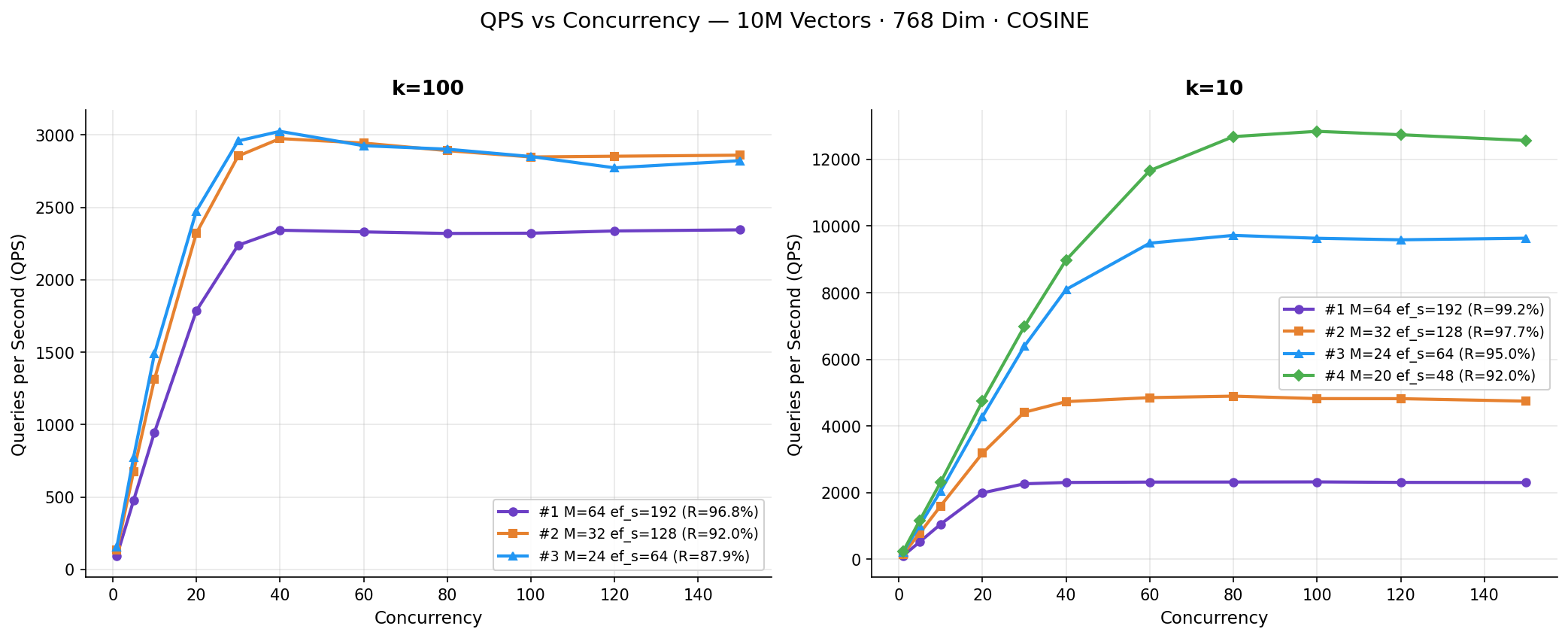
At k=10, the lighter configurations (Experiments #3 and #4) scale nearly linearly up to 60–80 concurrent clients before saturating. Experiment #4 demonstrates the benefit of a leaner graph: it achieves 5.5X higher peak QPS than Experiment #1 at k=10. At k=100, all configurations converge to a narrower throughput band (2,300–3,025 QPS). This shows that retrieving 100 neighbors dominates the per-query cost regardless of index parameters.
P99 and Average Latency vs Concurrency
As expected, increasing throughput adds queuing delay, and that leads to higher tail latencies.
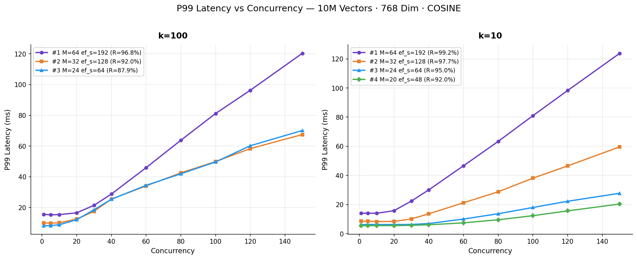
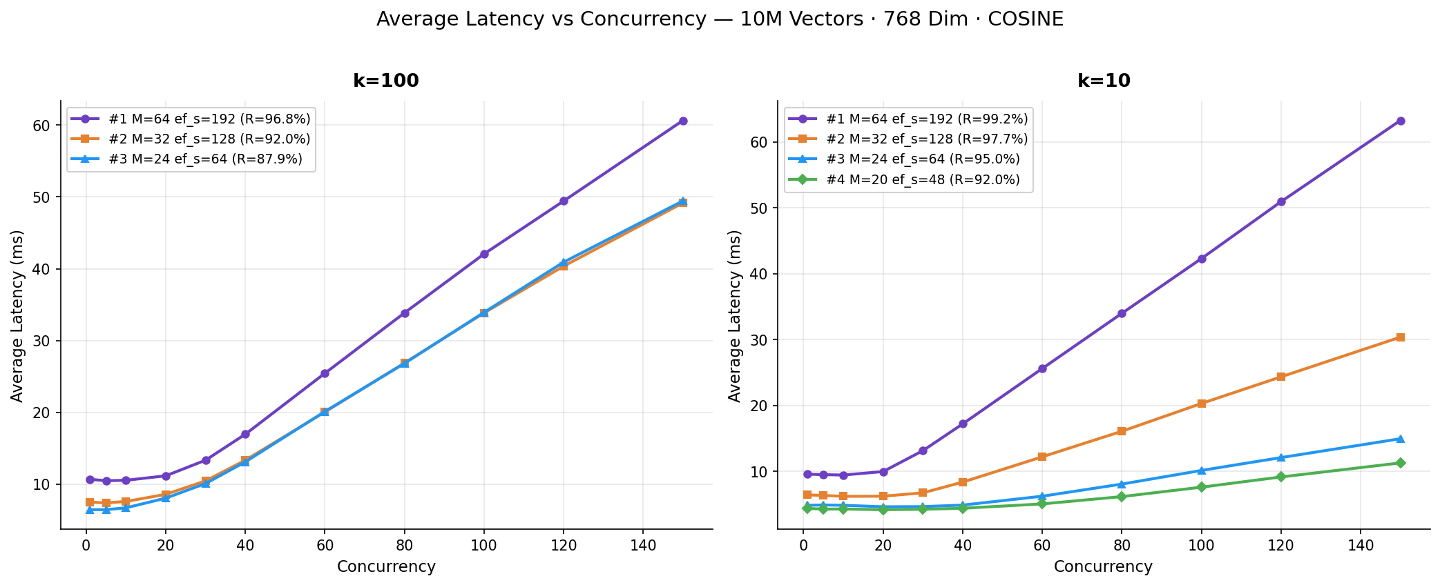
Lighter configurations start at dramatically lower baseline latencies. Experiment #4 maintains sub-6 ms P99 latency up to 30 concurrent clients, while Experiment #1 starts above 13 ms, even at concurrency 1. All configurations show latency rising proportionally once throughput saturates. This is the expected queuing behavior when the system is at capacity.
QPS vs P99 Latency (Pareto View)
Plotting throughput directly against tail latency provides a Pareto frontier of our benchmark configurations:
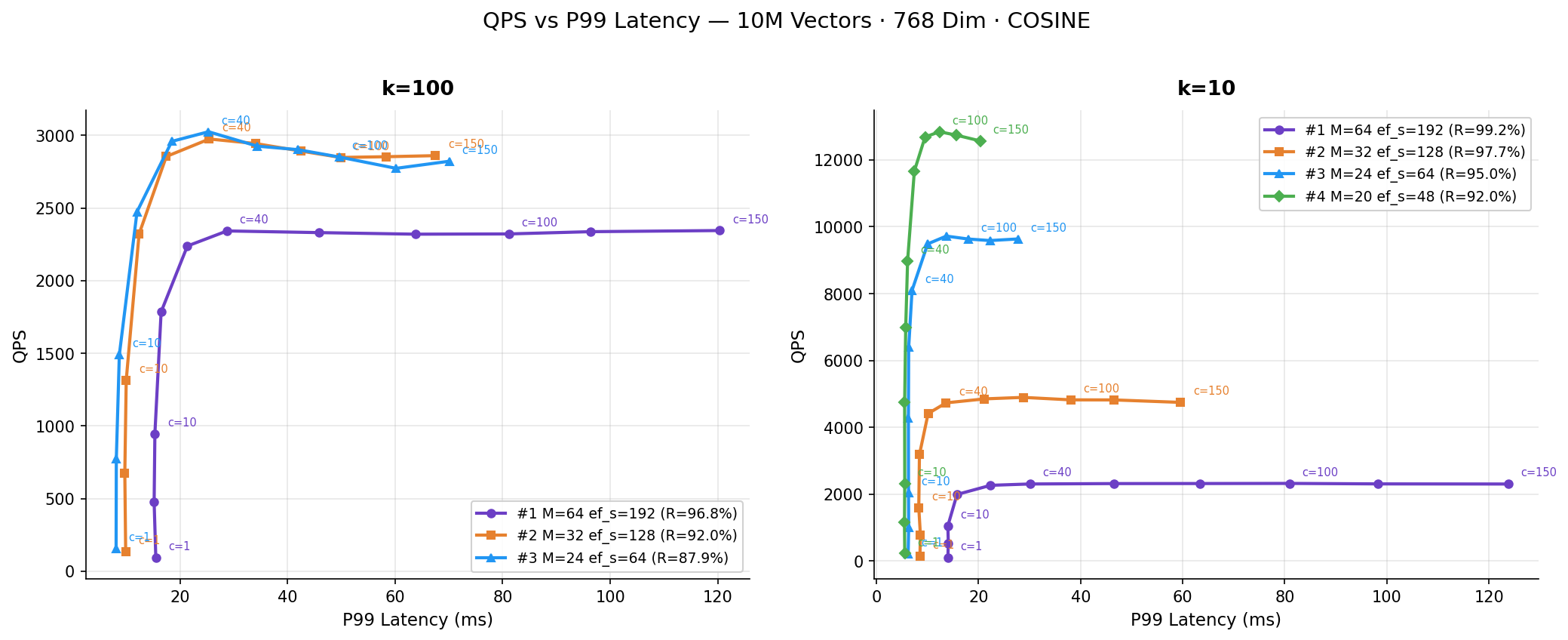
This view makes the operational trade-off easier to read than the concurrency charts alone. At k=10, Experiments #3 and #4 push the frontier outward, with much higher QPS at the same or lower tail latency. At k=100, the frontier is tighter, which again shows that returning more neighbors dominates the total cost per query.
Recall vs Peak QPS
Finally, plotting recall helps select the optimal index strategy based on business requirements:
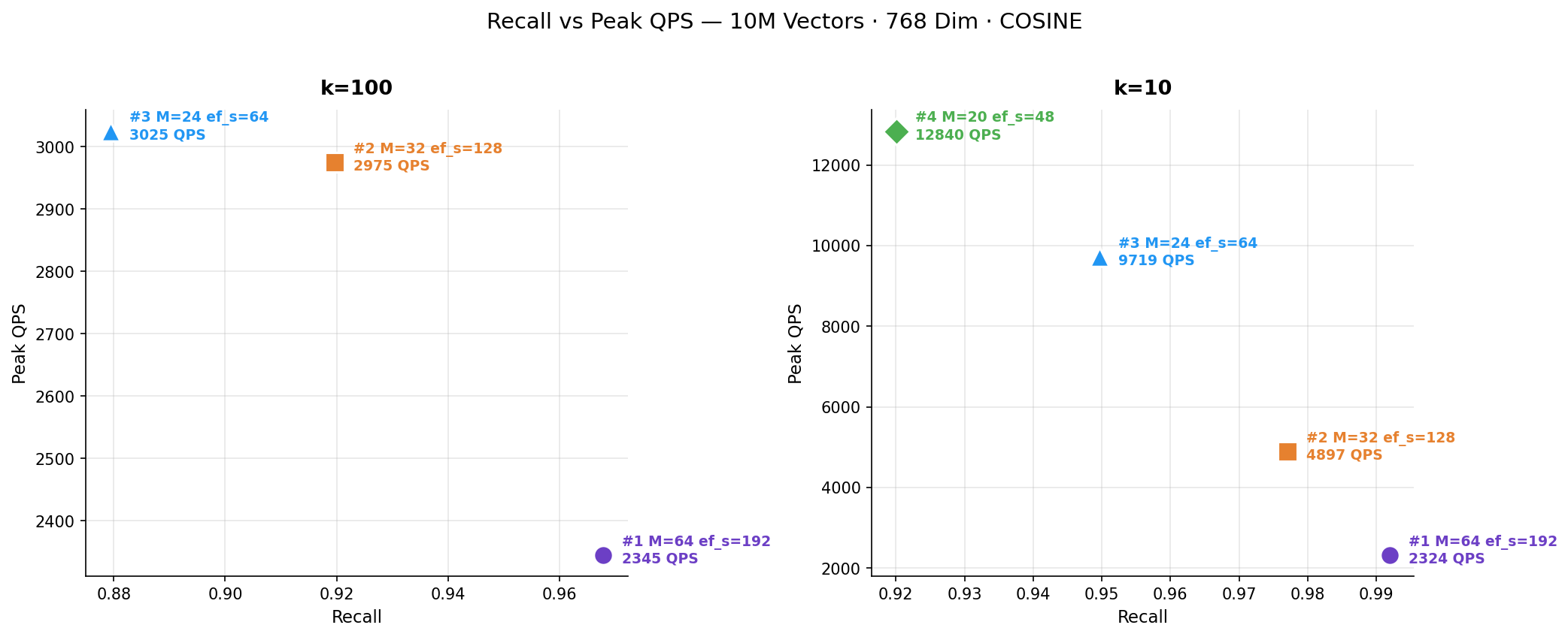
This chart summarizes the core choice in a single picture: should you spend compute on accuracy or throughput? Experiment #1 sits at the high-recall end, Experiment #4 at the high-throughput end, and Experiment #2 emerges as the practical middle ground for workloads that need both.
Scenario Analysis
With the charts above as a visual reference, let’s examine the three main usage scenarios that emerge from the data.
Scenario 1: Maximum Throughput
Experiments #3 (M=24, ef_search=64) and #4 (M=20, ef_search=48) target workloads where throughput is the primary objective and moderate recall is acceptable — for example, coarse candidate retrieval stages in recommendation pipelines or semantic deduplication.
At k=10, Experiment #4 reached a peak of 12,840 QPS at concurrency 100, with a serial P99 latency of just 5.5 ms and recall of 92.0%. Experiment #3 achieved 9,719 QPS with marginally better recall at 95.0% and a serial P99 of 6.0 ms.
Even at k=100, these lightweight configurations delivered competitive throughput: Experiment #3 peaked at 3,025 QPS (87.9% recall), which is comparable to the heavier configurations. Retrieval of 100 neighbors per query inherently requires more work, which limits the throughput range across all configurations.
Scenario 2: High Recall
Experiment #1 (M=64, ef_search=192) prioritizes accuracy for applications that cannot tolerate missed results (e.g., high-fidelity semantic search, retrieval-augmented generation [RAG] pipelines, or compliance-sensitive retrieval).
At k=10, the system delivered 99.2% recall and 99.1% nDCG — essentially indistinguishable from exact brute-force search. Peak QPS reached 2,324 with a serial P99 latency of 14.6 ms. At k=100, recall was 96.8% with 2,345 QPS and a serial P99 of 15.2 ms.
The higher latency and lower throughput are a direct consequence of the richer graph (64 connections per node) and wider search beam (192 candidates), which evaluate substantially more distance computations per query.
Scenario 3: Balanced
Experiment #2 (M=32, ef_search=128) takes the middle ground, offering strong recall with significantly better throughput than the high-recall configuration.
At k=10, it achieved 97.7% recall with 4,897 QPS — roughly double the throughput of Experiment #1, with only a 1.5 percentage-point recall reduction. The serial P99 was 8.7 ms. At k=100, recall was 92.0% with 2,975 QPS and a serial P99 of 9.6 ms.
This configuration represents a practical sweet spot for many production deployments where both recall and throughput matter.
Summary Tables
k=100
| Metric | #1 M=64 ef_s=192 | #2 M=32 ef_s=128 | #3 M=24 ef_s=64 |
|---|---|---|---|
| Peak QPS | 2,345 (c=150) | 2,975 (c=40) | 3,025 (c=40) |
| QPS @ c=10 | 947 | 1,314 | 1,489 |
| Serial P99 Latency | 15.2 ms | 9.6 ms | 7.8 ms |
| P99 Latency @ c=1 | 15.5 ms | 9.9 ms | 8.1 ms |
| P99 Latency @ c=100 | 81.2 ms | 49.9 ms | 49.6 ms |
| Recall | 96.8% | 92.0% | 87.9% |
| nDCG | 97.3% | 93.1% | 89.7% |
k=10
| Metric | #1 M=64 ef_s=192 | #2 M=32 ef_s=128 | #3 M=24 ef_s=64 | #4 M=20 ef_s=48 |
|---|---|---|---|---|
| Peak QPS | 2,324 (c=100) | 4,897 (c=80) | 9,719 (c=80) | 12,840 (c=100) |
| QPS @ c=10 | 1,054 | 1,602 | 2,046 | 2,311 |
| Serial P99 Latency | 14.6 ms | 8.7 ms | 6.0 ms | 5.5 ms |
| P99 Latency @ c=1 | 14.0 ms | 8.5 ms | 6.2 ms | 5.5 ms |
| P99 Latency @ c=100 | 81.0 ms | 38.1 ms | 18.0 ms | 12.3 ms |
| Recall | 99.2% | 97.7% | 95.0% | 92.0% |
| nDCG | 99.1% | 97.6% | 94.9% | 92.0% |
Key Takeaways
- k=10 vs k=100: At k=10, lighter index parameters yield massive throughput gains (up to 5.5X) with modest recall loss. At k=100, all configurations converge to a narrow QPS band (~1.3X range) because retrieving more neighbors dominates per-query cost.
- Recall trade-offs are favorable: At k=10, recall drops only 7.2 pp (99.2% to 92.0%) for a 5.5X QPS increase. At k=100, the trade-off is steeper: 8.9 pp for just 1.3X gain.
- Latency tracks index weight: Serial P99 drops from 14.6 ms to 5.5 ms at k=10, and from 15.2 ms to 7.8 ms at k=100, as lighter graphs require fewer distance computations.
- Saturation points differ: Experiments #1–#3 plateau around c=40–80; Experiment #4 scales further to c=100 before saturating, reflecting its lower per-query compute cost.
Conclusion
These results show that ScyllaDB Vector Search delivers strong performance even on a compact, five-node cluster with 10 million 768-dimensional vectors. A pair of r7g.2xlarge search nodes provides enough memory to hold the full HNSW index at f32 precision – without requiring any quantization. The three storage nodes with replication factor 3, combined with vector search nodes distributed across availability zones, also provide high availability. The system is designed to tolerate node failures without data loss or service interruption. Depending on the index configuration, the system can prioritize near-perfect recall (99.2% at k=10) or maximize throughput (12,840 QPS at k=10 with 92% recall), with practical balanced options in between.
This 10M scenario represents the accessible end of the scale. For workloads that push into hundreds of millions or billions of vectors, quantization, additional search nodes and larger instances extend the same architecture. See the ScyllaDB 1-billion-vector benchmark for results at extreme scale, and look for our upcoming 100-million-vector benchmark post.
At K=10, the performance bottleneck resides within the vector index nodes, leaving ScyllaDB with significant headroom. This means you can likely add a Vector Search index to your cluster and continue running a similar workload on your existing ScyllaDB infrastructure – without needing to scale your database nodes.
The full Jupyter notebook with interactive charts and all data is available in this repository.
Ready to try it yourself? Follow the ScyllaDB Vector Search Quick Start Guide to get started.