“Think back to some time when you were driving down the freeway, clipping right along about 5 miles above the limit even though the highway was busy, and then suddenly everyone slowed to a crawl and you had to stand on the brakes. Next came a quarter, a half, even a full mile of stop-and-go traffic. Finally, the pack broke up and you could come back to speed. But there was no cause to be seen. What happened to the traffic flaw?”
— Charles Wetherell, Etudes for Programmers
In the real world a “phantom traffic jam,” also called a “traffic wave,” is when there is a standing compression wave in automobile traffic, even though there is no accident, lane closure, or other incident that would lead to the traffic jam. A similar phenomenon is possible in computer networking or storage I/O, where your data can slow down for no apparent reason. Let’s look into what might cause such “phantom jams” in your data.
Introducing a Dispatcher to the Producer-Consumer Model
Consider there’s a thread that sends some messages into the hardware, say network packets into the NIC or I/O requests into the disk. The thread, called Producer, does this at some rate, P messages per second. The hardware, in turn, is capable of processing the messages at some other rate, C messages per second. This time, however, the Producer doesn’t have direct access to the Consumer’s input. Instead, the messages are put into some intermediate buffer or queue and then a third component, called Dispatcher, pushes those messages into their destination. Like this:
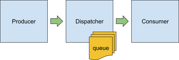
The Producer-Dispatcher-Consumer model
Being a software component, the Dispatcher may have limited access to the CPU power and is thus only “allowed” to dispatch the messages from its queue at certain points in time. Let’s assume that the dispatcher wakes up D times per second and puts several messages into the Consumer before getting off the CPU.
The Dispatcher component is not as artificial as it may seem. For example in the Linux kernel there’s I/O scheduler and network traffic shaper. In ScyllaDB, the database for data-intensive apps that require high performance and low latency, there’s Seastar’s reactor, etc. Having such an interposer allows the system architect to achieve various goals like access rights, priority classes, buffering, congestion control and many others.
Apparently, if P > C ( i.e. the Producer generates messages at a higher rate than the Consumer can process), then someone’s queue will grow infinitely – either the Dispatcher’s queue or the Consumer’s internal one. So further we’ll always assume that the C > P, i.e. the Consumer is fast enough to keep the whole system operating.
On the other hand, the Dispatcher is allowed to work at any rate it wants. Since it may put any amount of messages into the Consumer, its math would look like this. It takes L = 1 / C seconds for a Consumer to process a single message, Dispatcher sleep time between wake-ups is G = 1 / D, respectively it needs to put at least G / L = C / D messages into the Consumer so as not to disturb the message flow.
Why not put the whole queue accumulated so far? It’s possible, but there’s a drawback. If the Consumer is dumb and operates in FIFO mode (and in case it’s a hardware most likely it is dumb), the Dispatcher limits its flexibility in maintaining the incoming flow of messages. And since in ideal conditions the Consumer won’t process more than C / D requests, it makes sense to dispatch at most some-other-amount (larger than C / D) of requests per wake-up.
Adding some jitter to the data-flow chain
In the real world, however, none of the components is able to do its job perfectly. The Producer may try to generate the messages at the given rate, but this rate will only be visible in the long run. The real delay between messages will be different, being P on average. Similarly, the Consumer will process C messages per second, but the real delay between individual messages would vary around the 1 / C value. And, of course, the same is true for the Dispatcher – it will be woken up at unequal intervals, some below the 1 / D goal, some above, some are well above it. In the academic world there’s a nice model of this jittery behavior called the Poisson point process. In it, the events occur continuously, sequentially and independently at some given rate. Let’s try to disturb each of the components we have and see how it will affect its behavior.
To play with this model, here’s a simple simulating tool (written on C++) that implements the Producer, the Dispatcher and the Consumer and runs them over a virtual time axis for the given duration. Since it was initially written to model the way Seastar library dispatches the IO requests it uses a hard-coded Dispatcher wake-up rate of 2kHz and applies a multiplier of 1.5 to the maximum number of requests it is allowed to put into the Consumer as per above description (but both constants can be overridden with the command line options).
The tool CLI is as simple as
$ sim <run duration in seconds>
      <producer delays> <producer rate>
      <dispatcher delays>
      <consumer delays> <consumer rate>
Where “delays” arguments define how the simulator models the pauses between events in the respective component. In the end the tool prints the statistics about time it took for requests to be processed – the mean value, 95% and 99% percentiles and the maximum value.
First, let’s validate that the initial idea about perfect execution is valid, i.e. if all three components are running at precisely fixed rates the system is stable and processes all the requests. Since it’s a simulator, it can provide the perfect intervals between events. We’ll run the simulation at 200k messages per second rate and will do it for 10 virtual minutes. The command to run is
$ sim 600 uniform 200000 uniform uniform 200000The resulting timings would be
| mean | p95 | p99 | max |
| 0.5ms | 0.5ms | 0.5ms | 0.5ms |
Since the dispatcher runs at 2kHz rate, it can keep requests queued for about half-a-millisecond. Consumer rate of 200k messages doesn’t contribute much delay, so from the above timings we can conclude that the system is working as it should – all the messages generated by the Producer are consumed by the Consumer in a timely manner, the queue doesn’t grow.
Disturbing individual components
Next, let’s disturb the Producer and simulate the whole thing as if the input was not regular. Going forward, it’s better to run a series of experiments with increasing Producer rates and show the results on a plot. Here it is (mind the logarithmic vertical axis)
$ sim 600 poisson 200000 uniform uniform 200000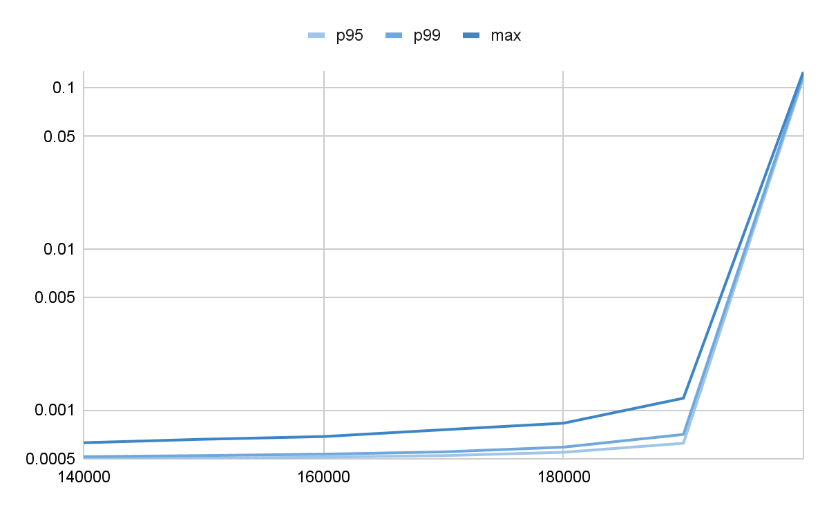
Pic.1 Messages latencies, jitter happens in the Producer
A disturbing, though not very unexpected thing happened. At extreme rates, the system cannot deliver the 0.5ms delay and requests spend more time in the Dispatcher’s queue than they do in the ideal case – up to 100ms. With the rates up to 90% of the peak, one the system seems to work, though the expected message latency is now somewhat larger than in the ideal case.
Well, how does the system work if the Consumer is disturbed? Let’s check
$ sim 600 uniform $rate uniform poisson 200000
Pic.2 Messages latencies, jitter happens in the Consumer
Pretty much the same, isn’t it. As the Producer rate reaches the Consumer’s maximum, the system delays requests but still, it works and doesn’t accumulate requests without bounds.
As you might have guessed, the most astonishing result happens if the Dispatcher is disturbed. Here’s how it looks.
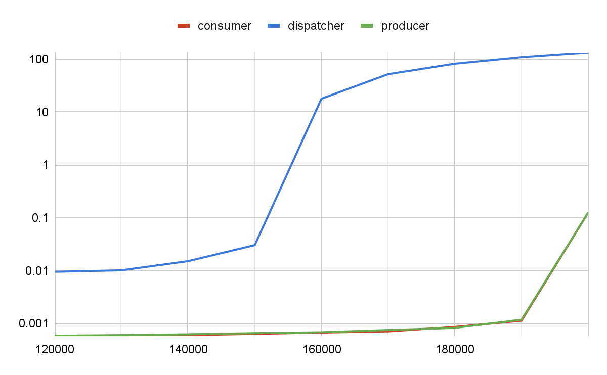
$ sim 600 uniform $rate poisson uniform 200000
Pic.3 Messages latencies, jitter happens in the Dispatcher
Now this is really weird. Despite the Dispatcher trying to compensate for the jitter by serving 1.5 times more requests into the Consumer per tick than it’s estimated by the ideal model, the effect on disturbing the Dispatcher is the largest. The request timings are 1k times of what they were when the Consumer or the Producer experienced the jitter. In fact, if we check the simulation progress in more detail, it becomes clear that at the rate of 160k requests per second, the system effectively stops maintaining the incoming message flow and the Dispatcher queue grows infinitely.
To emphasize the difference between the effect the jitter has on each of the components, here’s how the maximum latency changes with the increase of the Producer rate. Different plots correspond to the component that experiences jitter.
Pic.4 Comparing jitter effect on each of the components
The Dispatcher seemed to be the least troublesome component that didn’t have any built-in limiting factors. Instead, there was an attempt to over-dispatch the Consumer with requests in case of any delay in service. Still the imperfection of the Dispatcher has the heaviest effect on the system performance. Not only jitter in the Dispatcher renders higher delays in messages processing, but also the maximum throughput of the system is mainly determined by the Dispatcher, not by the Consumer or the Producer.
Discovering the “effective dispatch rate”
This observation brings us to the idea of the effective dispatch rate – the maximum number of requests per second such a system may process. Apparently, this value is determined by the Consumer rate and depends on the behavior of the Dispatcher which, in turn, has two parameters – dispatch frequency and the over-dispatch multiplier. Using the simulation tool, it is possible to get this rate for different frequencies (actually, since the tool is seastar-centric it accepts the dispatch period duration, not the frequency itself) and multipliers. The plot below shows how the effective rate (the Y-axis) changes with the dispatch multiplier value (the X-axis) in 3 different dispatch rates – quarter, half and two milliseconds.
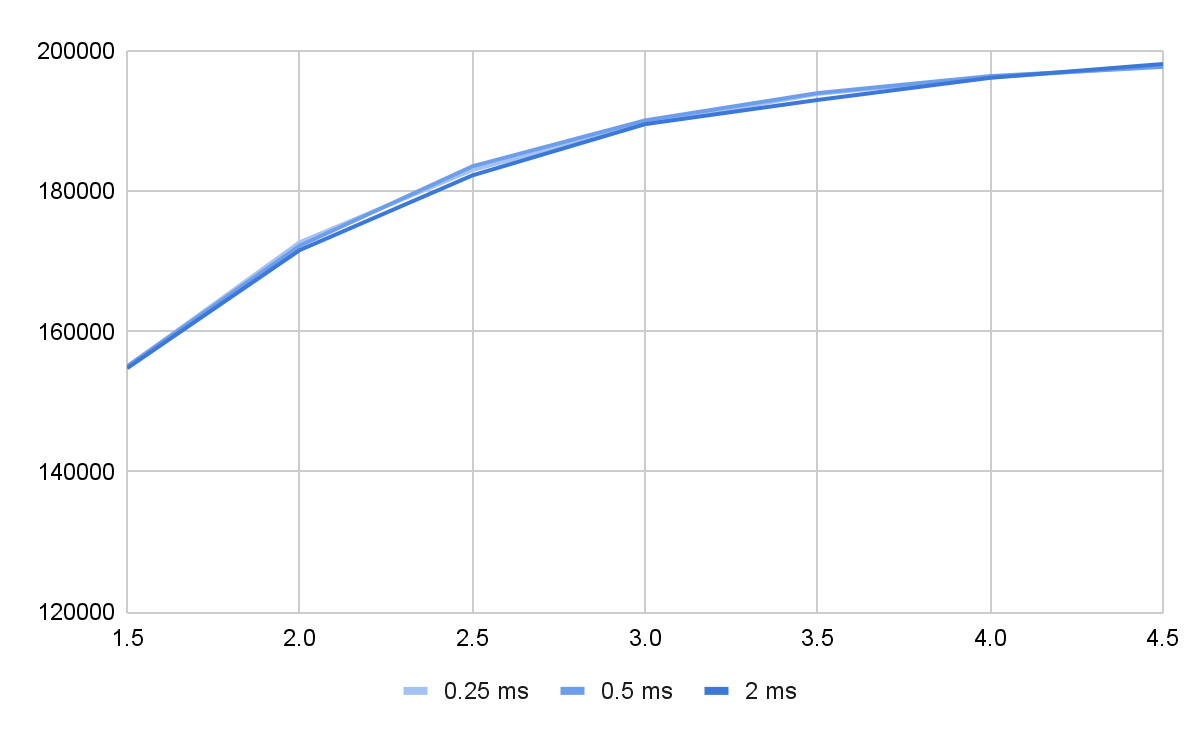
Pic. 5 Effective dispatch rate of different Dispatcher wake-up periods
As seen on the plot, the frequency of Dispatcher wake ups doesn’t matter. What affects the effective dispatch rate is the over-dispatching level – the more requests the Dispatcher puts into the Consumer, the better it works. It seems like that’s the solution to the problem. However, before jumping to this conclusion, we should note that the more requests are sitting in the Consumer simultaneously, the longer it takes for it to process it, and the worse end latencies may occur. Unfortunately, this is where the simulation boundary is. If we check this with the simulator, we’ll see even at the multiplier of 4.0, the end latency doesn’t become worse. But that’s because what grows is the in-Consumer latency, and since it’s much lower than the in-Dispatcher one, the end latency doesn’t change a lot. The ideal Consumer is linear – it takes exactly twice as much time to process two times more requests. Real hardware consumers (disks, NICs, etc.) do not behave like that. Instead, as the internal queue grows, the resulting latency goes up worse than linearly – so over-dispatching the Consumer will render higher latencies.
The Producer-Consumer model is quite a popular programming pattern. Although the effect was demonstrated in a carefully prepared artificial environment, it may reveal itself at different scales in real systems as well. Fighting one can be troublesome indeed, but in this particular case it’s worth saying that forewarned is forearmed. The key requirement for its disclosure is the elaborated monitoring facilities and profound understanding of the system components.
Discover More About ScyllaDB
ScyllaDB is a monstrously fast and scalable NoSQL database designed to provide optimal performance and ease of operations. You can learn more about its design by checking out its architecture on our website, or download our white paper on the Seven Design Principles behind ScyllaDB.