This blog post is based on a talk I gave last month at the third annual ScyllaDB Summit in San Francisco. It explains how ScyllaDB ensures that ingestion of data proceeds as quickly as possible, but not quicker. It looks into the existing flow-control mechanism for tables without materialized views, and into the new mechanism for tables with materialized views, which is introduced in ScyllaDB Open Source 3.0.
Introduction
In this post we look into ingestion of data into a ScyllaDB cluster. What happens when we make a large volume of update (write) requests?
We would like the ingestion to proceed as quickly as possible but without overwhelming the servers. An over-eager client may send write requests faster than the cluster can complete earlier requests. If this is only a short burst of requests, ScyllaDB can absorb the excess requests in a queue or numerous queues distributed throughout the cluster (we’ll look at the details of these queues below). But had we allowed the client to continue writing at this excessive rate, the backlog of uncompleted writes would continue to grow until the servers run out of memory and possibly crash. So as the backlog grows, we need to find a way for the server to tell the client to slow down its request rate. If we can’t slow down the client, we have to start failing new requests.
Cassandra’s CQL protocol does not offer any explicit flow-control mechanisms for the server to slow down a client which is sending requests faster than the server can handle them. We only have two options to work with: delaying replies to the client’s requests, and failing them. How we can use these two options depends on what drives the workload: We consider two different workload models — a batch workload with bounded concurrency, and an interactive workload with unbounded concurrency:
- In a batch workload, a client application wishes to drive the server at 100% utilization for a long time, to complete some predefined amount of work. There is a fixed number of client threads, each running a request loop: preparing some data, making a write request, and waiting for its response. The server can fully control the request rate by rate-limiting (delaying) its replies: If the server only sends N replies per second, the client will only send N new requests per second. We call this rate-limiting of replies, or throttling.
- In an interactive workload, the client sends requests driven by some external events (e.g., activity of real users). These requests can come at any rate, which is unrelated to the rate at which the server completes previous requests. For such a workload, if the request rate is at or below the cluster’s capacity, everything is fine and the request backlog will be mostly empty. But if the request rate is above the cluster’s capacity, the server has no way of slowing down these requests and the backlog grows and grows. If we don’t want to crash the server (and of course, we don’t), we have no choice but to return failure for some of these requests.
When we do fail requests, it’s also important how we fail: We should fail fresh new, not yet handled, client requests. It’s a bad idea to fail requests to which we had already devoted significant work — if the server spends valuable CPU time on requests which will end up being failed anyway, throughput will lower. We use the term admission control for a mechanism which fails a new request when it believes the server will not have the resources needed to handle the request to completion.
For these reasons ScyllaDB utilizes both throttling and admission control. Both are necessary. Throttling is a necessary part of handling normal batch workloads, and admission control is needed for unexpected overload situations. In this post, we will focus on the throttling part.
We sometimes use the term backpressure to describe throttling, which metaphorically takes the memory “pressure” (growing queues) which the server is experiencing, and feeds it back to the client. However, this term may be confusing, as historically it was used for other forms of flow control, not for delaying replies as a mechanism to limit the request rate. In the rest of this document I’ll try to avoid the term “backpressure” in favor of other terms like throttling and flow control.
Above we defined two workload models — interactive and and batch workloads. We can, of course, be faced by a combination of both. Moreover, even batch workloads may involve several independent batch clients, starting at different times and working with different concurrencies. The sum of several such batch workloads can be represented as one batch workload with a changing client concurrency. E.g., a workload can start with concurrency 100 for one minute, then go to concurrency 200 for another minute, etc. Our flow control algorithms need to reasonably handle this case as well, and react to a client’s changing concurrency. As an example, consider that the client doubled the number of threads. Since the total number of writes the server can handle per second remains the same, now each client thread will need to send requests at half the rate it sent earlier when there were just half the number of threads.
The problem of background writes
Let’s first look at writes to regular ScyllaDB tables which do not have materialized views. Later we can see how materialized views further complicate matters.
A client sends an update (a write request) to a coordinator node, which sends the update to RF replicas (RF is the replication factor — e.g., 3). The coordinator then waits for first CL (consistency level — e.g., 2) of those writes to have completed, at which point it sends a reply to the client, saying that the desired consistency-level has been achieved. The remaining ongoing writes to replicas (RF-CL — in the above examples =1 remaining write) will then continue “in the background”, i.e., after the response to the client, and without the client waiting for them to finish.
The problem with these background writes is that a batch workload, upon receiving the server’s reply, will send a new request before these background writes finish. So if new writes come in faster than we can finish background writes, the number of these background writes can grow without bound. But background writes take memory, so we cannot allow them to grow without bound. We need to apply some throttling to slow the workload down.
The slow node example
Before we explain how ScyllaDB does this throttling, it is instructive to look at one concrete — and common — case where background writes pile up and throttling becomes necessary.
This is the case where one of the nodes happens to be, for some reason, consistently slower than the others. It doesn’t have to be much slower — even a tiny bit slower can cause problems:
Consider, for example, three nodes and a table with RF=3, i.e., all data is replicated on all three nodes, so all writes need to go to all three. Consider than one node is just 1% slower: Two of the nodes can complete 10,000 replica writes per second, while the third can only complete 9,900 replica writes per second. If we do CL=2 writes, then every second 10,000 of these writes can complete after node 1 and 2 completed their work. But since node 3 can only finish 9,900 writes in this second, we will have added 100 new “background writes” waiting for the write to node 3 to complete. We will continue to accumulate 100 additional background writes each second and, for example, after 100 seconds we will have accumulated 10,000 background writes. And this will continue until we run out of memory, unless we slow down the client to only 9,900 writes per second (and in a moment, we’ll explain how). It is possible to demonstrate this and similar situations in real-life ScyllaDB clusters. But to make it easier to play with different scenarios and flow-control algorithms, we wrote a simple simulator. In the simulator we can exactly control the client’s concurrency, the rate at which each replica completes write requests, and then graph the lengths of the various queues, the overall write performance, and so on, and investigate how those respond to different throttling algorithms.
In our simple “slow node” example, we see the following results from the simulator:
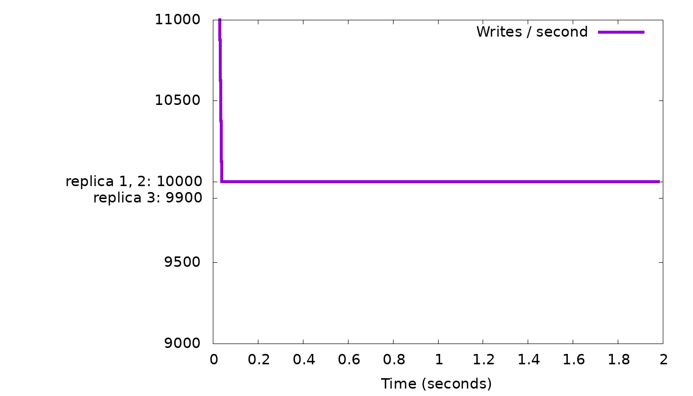
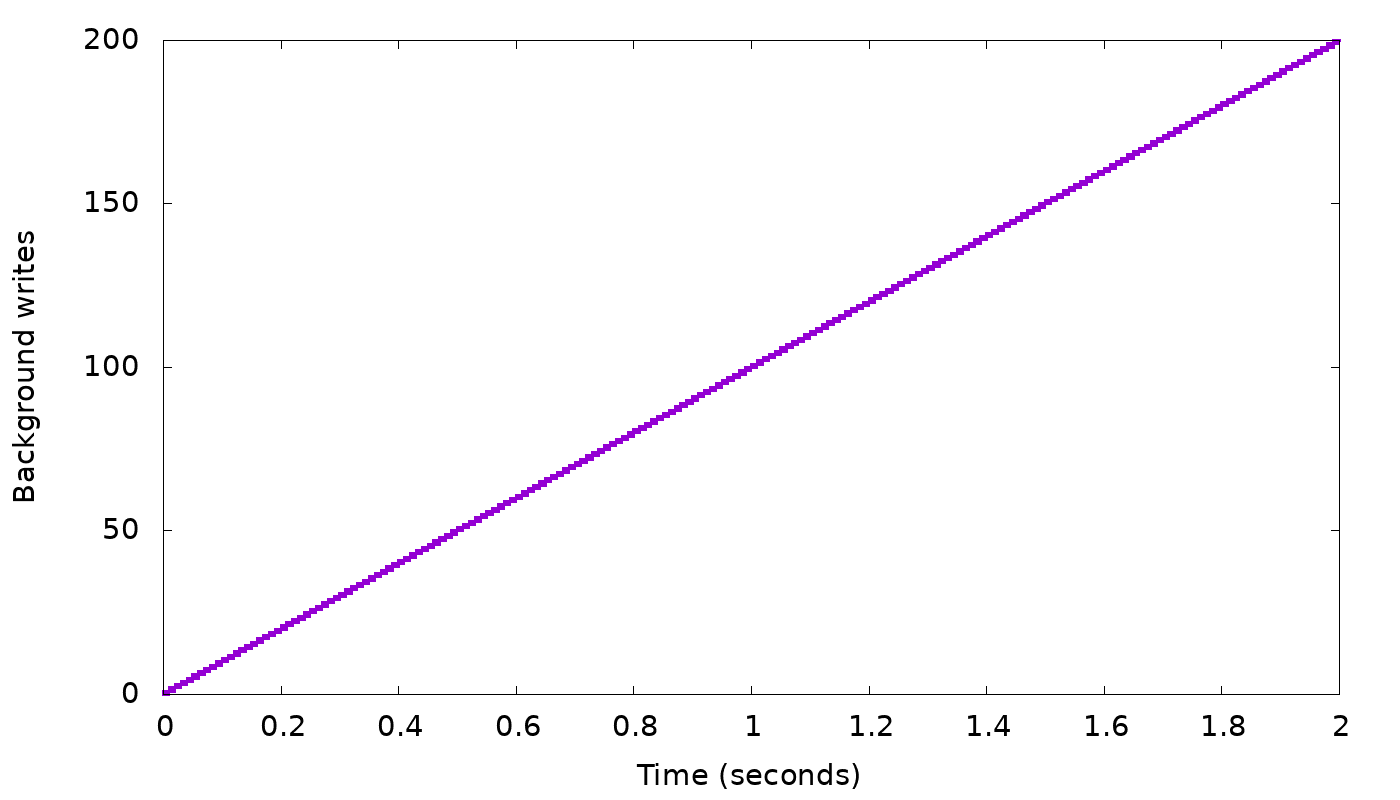
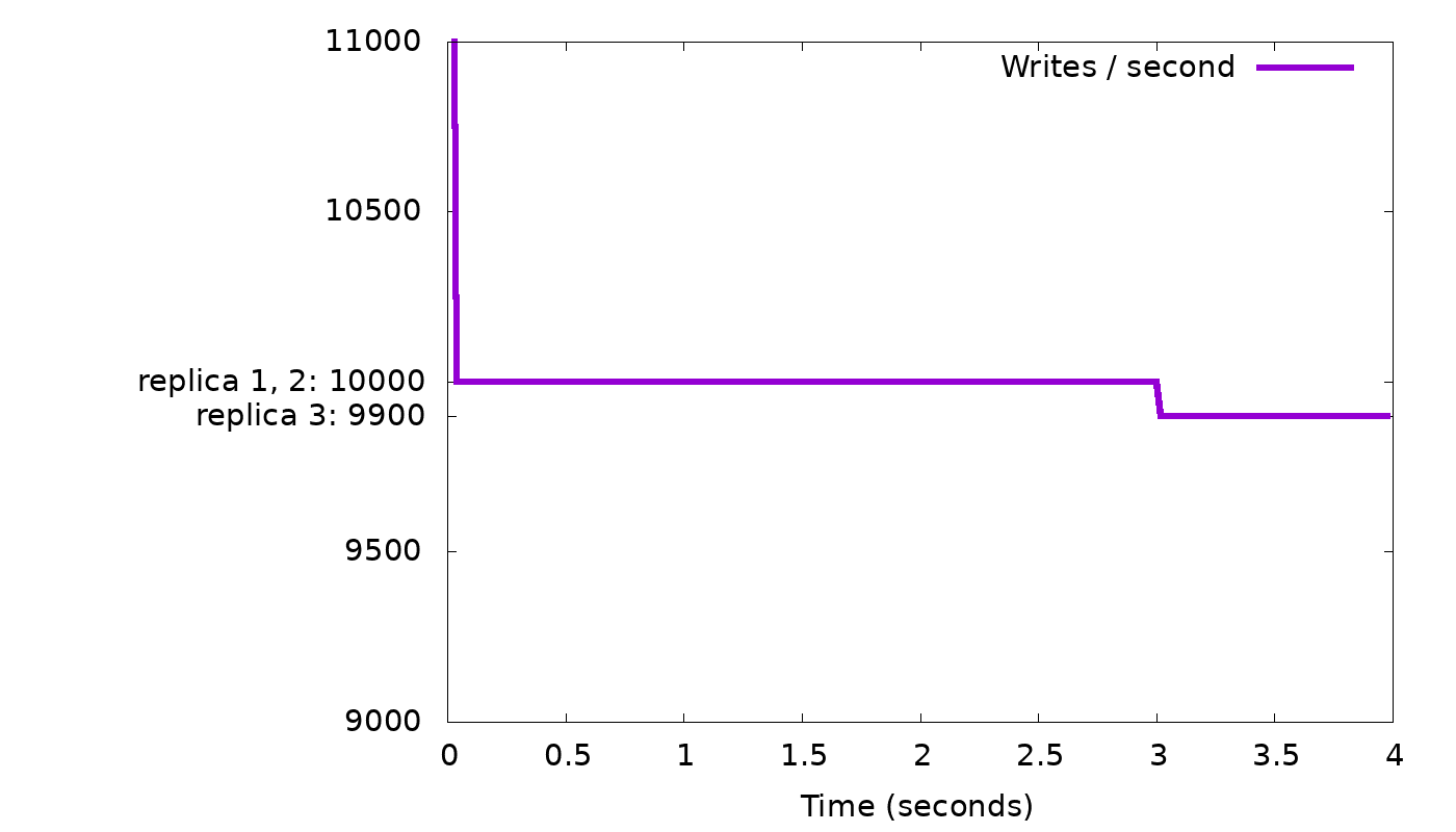
In the top graph, we see that a client with fixed concurrency (arbitrarily chosen as 50 threads) writing with CL=2 will, after a short burst, get 10,000 replies each second, i.e., the speed of the two fastest nodes. But while staying at that speed, we see in the bottom graph that the backlog of background writes grows continuously — 100 every second, as we suspected. We need to slow down the client to curb this growth.
It’s obvious from the description above that any consistent difference in node performance, even much smaller than 1%, will eventually cause throttling to be needed to avoid filling the entire memory with backlogged writes. In real-life such small performance differences do happen in clouds, e.g., because some of the VMs have busier “neighbors” than others.
Throttling to limit background writes
ScyllaDB applies a simple, but effective, throttling mechanism: When the total amount of memory that background writes are currently using goes over some limit — currently 10% of the shard’s memory — the coordinator starts throttling the client by no longer moving writes from foreground to background mode. This means that the coordinator will only reply when all RF replica writes have completed, with no additional work left in the background. When this throttling is on, the backlog of background writes does not continue to grow, and replies are only sent at the rate we can complete all the work, so a batch workload will slow down its requests to the same rate.
It is worth noting that when throttling is needed, the queue of background writes will typically hover around its threshold size (e.g., 10% of memory). When a flow-control algorithm always keeps a full queue, it is said to suffer from the bufferbloat problem. The typical bufferbloat side-effect is increased latency, but happily in our case this is not an issue: The client does not wait for the background writes (since the coordinator has already returned a reply), so the client will experience low latency even when the queue of background writes is full. Nevertheless, the full queue does have downsides: it wastes memory and it prevents the queue from absorbing writes to a node that temporarily goes down.
Let’s return to our “slow node” simulation from above, and see how this throttling algorithm indeed helps to curb the growth of the backlog of background writes:

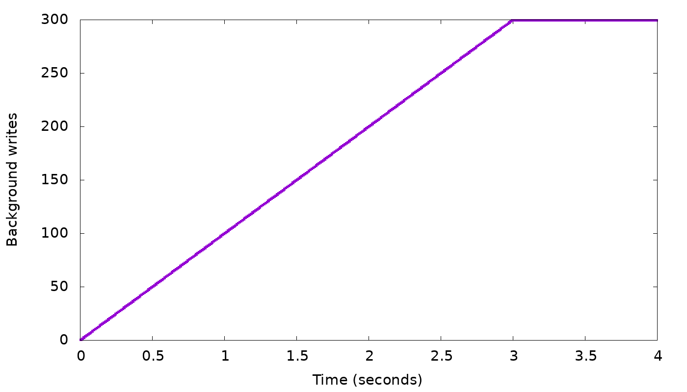
As before, we see in the top graph that the server starts by sending 10,000 replies per second, which is the speed of the two fastest nodes (remember we asked for CL=2). At that rate, the bottom graph shows we are accruing a backlog of 100 background writes per second, until at time 3, the backlog has grown to 300 items. In this simulation we chose 300 as background write limit (representing the 10% of the shard’s memory in real ScyllaDB). So at that point, as explained above, the client is throttled by having its writes wait for all three replica writes to complete. Those will only complete at rate of 9,900 per second (the rate of the slowest node), so the client will slow down to this rate (top graph, starting from time 3), and the background write queue will stop growing (bottom graph). If the same workload continues, the background write queue will remain full (at the threshold 300) — if it temporarily goes below the threshold, throttling is disabled and the queue will start growing back to the threshold.
The problem of background view updates
After understanding how ScyllaDB throttles writes to ordinary tables, let’s look at how ScyllaDB throttles writes to materialized views. Materialized views were introduced in ScyllaDB 2.0 as an experimental feature — please refer to this blog post if you are not familiar with them. They are officially supported in ScyllaDB Open Source Release 3.0, which also introduces the throttling mechanism we describe now, to slow down ingestion to the rate at which ScyllaDB can safely write the base table and all its materialized views.
As before, a client sends a write requests to a coordinator, and the coordinator sends them to RF (e.g., 3) replica nodes, and waits for CL (e.g., 2) of them to complete, or for all of them to complete if the backlog of background write reached the limit. But when the table (also known as the base table) has associated materialized views, each of the base replicas now also sends updates to one or more paired view replicas — other nodes holding the relevant rows of the materialized views.
The exact details of which updates we send, where, and why is beyond the scope of this post. But what is important to know here is that the sending of the view updates always happens asynchronously — i.e., the base replica doesn’t wait for it, and therefore the coordinator does not wait for it either — only the completion of enough writes to the base replicas will determine when the coordinator finally replies to the client.
The fact that the client does not wait for the view updates to complete has been a topic for heated debate ever since the materialized view feature was first designed for Cassandra. The problem is that if a base replica waits for updates to several view replicas to complete, this hurts high availability which is a cornerstone of Cassandra’s and ScyllaDB’s design.
Because the client does not wait for outstanding view updates to complete, their number may grow without bound and use unbounded amounts of memory on the various nodes involved — the coordinator, the RF base replicas and all the view replicas involved in the write. As in the previous section, here too we need to start slowing down the client, until the rate when the system completes background work at the same rate as new background work is generated.
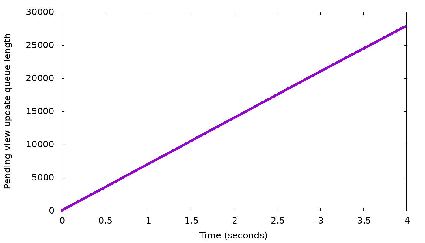
To illustrate the problem ScyllaDB needed to solve, let’s use our simulator again to look at a concrete example, continuing the same scenario we used above. Again we have three nodes, RF=3, client with 50 threads writing with CL=2. As before two nodes can complete 10,000 base writes per second, and the third only 9,900. But now we introduce a new constraint: the view updates add considerable work to each write, to the point that the cluster can now only complete 3,000 writes per second, down from the 9,900 it could complete without materialized views. The simulator shows us (top graph below) that, unsurprisingly, without a new flow-control mechanism for view writes the client is only slowed down to 9,900 requests per second, not to 3,000. The bottom graph shows that at this request rate, the memory devoted to incomplete view writes just grows and grows, by as many as 6,900 (=9,900-3,000) updates per second:
So, what we need now is to find a mechanism for the coordinator to slow down the client to exactly 3,000 requests per second. But how do we slow down the client, and how does the coordinator know that 3,000 is the right request rate?
Throttling to limit background view updates
Let us now explain how ScyllaDB 3.0 throttles the client to limit the backlog of view updates. We begin with two key insights:
- To slow down a batch client (with bounded concurrency), we can add an artificial delay to every response. The longer the delay is, the lower the client’s request rate will become.
- The chosen delay influences the size of the view-update backlog: Picking a higher delay slows down the client and slows the growth of the view update backlog, or even starts reducing it. Picking a lower delay speeds up the client and increases the growth of the backlog.
Basically, our plan is to devise a controller, which changes the delay based on the current backlog, trying to keep the length of the backlog in a desired range. The simplest imaginable controller, a linear function, works amazingly well:
(1) delay = α ⋅ backlog
Here α is any constant. Why does this deceptively-simple controller work?
Remember that if delay is too small, backlog starts increasing, and if delay is too large, the backlog starts shrinking. So there is some “just right” delay, where the backlog size neither grows nor decreases. The linear controller converges on exactly this just-right delay:
- If delay is lower than the just-right one, the client is too fast, the backlog increases, so according to our formula (1), we will increase delay.
- If delay is higher than the just-right one, the client is too slow, the backlog shrinks, so according to (1), we will decrease delay.
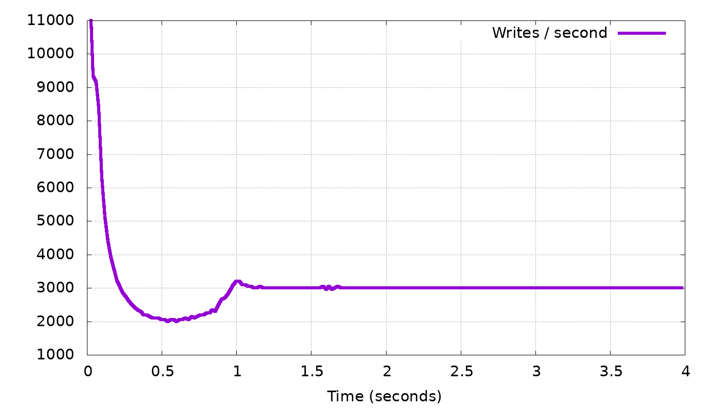
Let’s add to our simulator the ability to delay responses by a given delay amount, and to vary this delay according to the view update backlog in the base replicas, using formula (1). The result of this simulation looks like this:
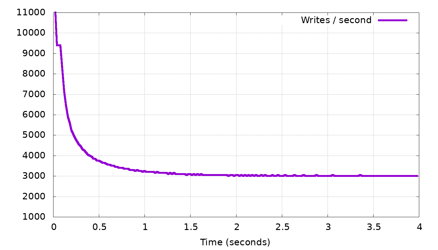
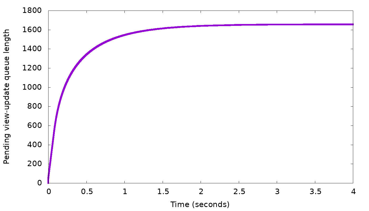
In the top graph, we see the client’s request rate gradually converging to exactly the request rate we expected: 3,000 requests per second. In the bottom graph, the backlog length settles on about 1600 updates. The backlog then stops growing any more — which was our goal.
But why did the backlog settle on 1600, and not on 100 or 1,000,000? Remember that the linear control function (1) works for any α. In the above simulation, we took α = 1.0 and the result was convergence on backlog=1600. If we change α, the delay to which we converge will still have to be the same, so (1) tells us that, for example, if we double α to 2.0, the converged backlog will halve, to 800. In this manner, if we gradually change α we can reach any desired backlog length. Here is an example, again from our simulator, where we gradually changed α with the goal of reaching a backlog length of 200:
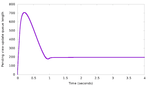
Indeed, we can see in the lower graph that after over-shooting the desired queue length 200 and reaching 700, the controller continues to increase to decrease the backlog, until the backlog settles on exactly the desired length — 200. In the top graph we see that as expected, the client is indeed slowed down to 3,000 requests per second. Interestingly in this graph, we also see a “dip”, a short period where the client was slowed down even further, to just 2,000 requests per second. The reason for this is easy to understand: The client starts too fast, and a backlog starts forming. At some point the backlog reached 700. Because we want to decrease this backlog (to 200), we must have a period where the client sends less than 3,000 requests per second, so that the backlog would shrink.
In controller-theory lingo, the controller with the changing α is said to have an integral term: the control function depends not just on the current value of the variable (the backlog) but also on the previous history of the controller.
In (1), we considered the simplest possible controller — a linear function. But the proof above that it converges on the correct solution did not rely on this linearity. The delay can be set to any other monotonically-increasing function of the backlog:
(2) delay = f(backlog / backlog0) ⋅ delay0
(where backlog0 is a constant with backlog units, and delay0 is a constant with time units).
In ScyllaDB 3.0 we chose this function to be a polynomial, selected to allow relatively-high delays to be reached without requiring very long backlogs in the steady state. But we do plan to continue improving this controller in future releases.
Conclusion
A common theme in ScyllaDB’s design, which we covered in many previous blog posts, is the autonomous database, a.k.a. zero configuration. In this post we covered another aspect of this theme: When a user unleashes a large writing job on ScyllaDB, we don’t want him or her to need to configure the client to use a certain speed or risk overrunning ScyllaDB. We also don’t want the user to need to configure ScyllaDB to limit an over-eager client. Rather, we want everything to happen automatically: The write job should just just run normally without any artificial limits, and ScyllaDB should automatically slow it down to exactly the right pace — not too fast that we start piling up queues until we run out of memory, but also not too slow that we let available resources go to waste.
In this post, we explained how ScyllaDB throttles (slows down) the client by delaying its responses, and how we arrive at exactly the right pace. We started with describing how throttling works for writes to ordinary tables — a feature that had been in ScyllaDB for well over a year. We then described the more elaborate mechanisms we introduce in ScyllaDB 3.0 for throttling writes to tables with materialized views. For demonstration purposes, we used a simulator for the different flow-control mechanisms to better illustrate how they work. However, these same algorithms have also been implemented in ScyllaDB itself — so go ahead and ingest some data! Full steam ahead!

Worry Free Ingestion at ScyllaDB Summit 2018
Nad’av Harel presented on the topic of Worry-Free Ingestion: Flow Control of Writes at ScyllaDB Summit 2018. You can read his slide presentation and browse all the other ScyllaDB Summit 2018 sessions in our Tech Talks section, or watch the video below.
Next Steps
- Learn more about ScyllaDB from our product page.
- Learn more about ScyllaDB Open Source Release 3.0.
- See what our users are saying about ScyllaDB.
- Download ScyllaDB. Check out our download page to run ScyllaDB on AWS, install it locally in a Virtual Machine, or run it in Docker.
Editor’s Note: This blog has been revised to reflect that this feature is now available in ScyllaDB Open Source Release 3.0.