
Stop overprovisioning; true elastic scale lets you increase capacity fast, without latency spikes or wasted spend
There’s a pattern I keep seeing when talking to teams about database costs (admittedly, a pattern I’ve been susceptible to myself).
They size for the peak.
Then they run a subset of utilization of that for the rest of the time.
Inevitably, six months later someone asks “Why is our database so expensive?”
Sound familiar?
I’ve written about this before, especially in the context of DynamoDB pricing bill shock. But it’s not (just) a DynamoDB problem…
It’s a general database problem.
Overprovisioning is the silent budget killer.
The Overprovisioning Trap
Let’s say your workload looks something like this:
- Morning ramp-up
- Midday peak
- Afternoon dip
- Evening spike
- Overnight quiet
Pretty normal, right? But most databases force you to provision for the worst hour of the day. So, you end up paying peak prices all day long. That’s not elasticity; that’s overprovisioning in a nutshell.
Some teams try to fix this with autoscaling, reserved capacity, or on-demand bursts. That helps, but it still doesn’t fully solve the problem.
To understand why, we need to look at what paying only for what you need actually looks like.
What Paying for What You Need Actually Looks Like
This is where the ScyllaDB cost calculator becomes useful.
Instead of guessing capacity for peaks, you model your workload hour-by-hour. You baseline your traffic, account for spikes, batch jobs, or even unpredictable workloads.
 The calculator then splits your workload into:
- Baseline capacity which always on
- Flex capacity only when needed
It automatically finds the lowest-cost mix of pricing models (what we call hybrid pricing).
In other words, you stop paying for peak all the time and only pay for peaks when they happen.
A Real World Retail Example
The calculator includes a number of pre-built scenarios that help illustrate these savings, especially if switching from DynamoDB.

The retail example models a baseline of 10K ops/sec for reads + 10K ops/sec for writes. There’s a peak of 500K ops/sec for just reads (think flash sale or ad campaign) and a peak duration of 2 hours per day. It also has a small storage footprint of 0.5 TB across 5 regions. For each of those regions, it also deploys a cache using DAX (DynamoDB Accelerator).

The traffic pattern shows a workload that’s flat most of the day, then spikes 50x during a promotion window. That’s precisely the kind of pattern that breaks budget assumptions.
Here’s what that costs:
- DynamoDB [$1.6M/year]
- ScyllaDB [$271K/year]
That’s a gigantic +$1.3M/year difference! It’s not because the workload is smaller. It’s because you’re paying for peak capacity around the clock, not to mention being penalized for using more than 1 region within DynamoDB and exorbitant costs for caching. [more on DynamoDB cost multipliers]
Why This Matters More at Scale
At a small scale, overprovisioning is annoying. At monster scale, it’s catastrophic.
For example, take the sports scenario modeled in the calculator: real-time event data with write-heavy and spiky traffic. Storage is 3 TB with reads around 150 – 500K ops/sec (driven by live game traffic) and writes up to 1M ops/sec during match events.

Here’s what that costs:
- DynamoDB [$16.6M/year]
- ScyllaDB [$633K/year]
That is an eye-blistering multi-million dollar difference – perhaps enough to ruin your entire cloud infrastructure budget.
Planned Peaks and Unplanned Peaks
Real workloads are messy. Some peaks can be anticipated (flash sales, game days, product launches), but many cannot. Some are just the daily rhythms: morning ramp, midday peaks, and overnight dips.
Billing doesn’t differentiate between these peaks. If your platform cannot react fast enough, your only safe option is to… (You’re getting it now)…overprovision. And that’s precisely why costs explode.
Take the advertising scenario: read-heavy traffic where demand can jump from around 4M reads/sec to over 10M reads/sec.

- DynamoDB (provisioned for peak) [$10.6M/year]
- ScyllaDB (hybrid baseline + flex) [$961K/year]
That’s a +$9.6M/year delta, largely driven by one question: Do you pay for the spike all year, or only when the spike occurs?
Daily Patterns with Subtle Overspend
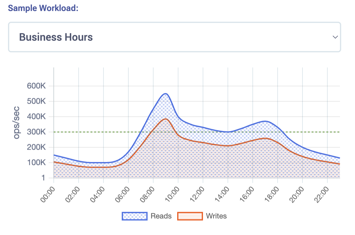
Dor’s keynote calls out a common “diurnal” traffic pattern. That’s what we see in many production systems: business hours demand reduced to overnight lulls.
The social media scenario models business hours across multiple regions (therein lies another cost lever in DynamoDB, as I covered in this blog).

The morning and afternoon peaks are predictable. However, the swing between high and low periods after hours, even if you provision the reads (you can’t provision replicated writes in DynamoDB) still produces a massive spend:
- DynamoDB (provisioned, multi-region) [$11.0M/year]
- ScyllaDB (hybrid baseline + flex) [$591K/year]
ScyllaDB handles this elegantly, scaling down overnight and coming back up in the morning with zero impact to P99 latency. This way, you stop paying for peaks around the clock.
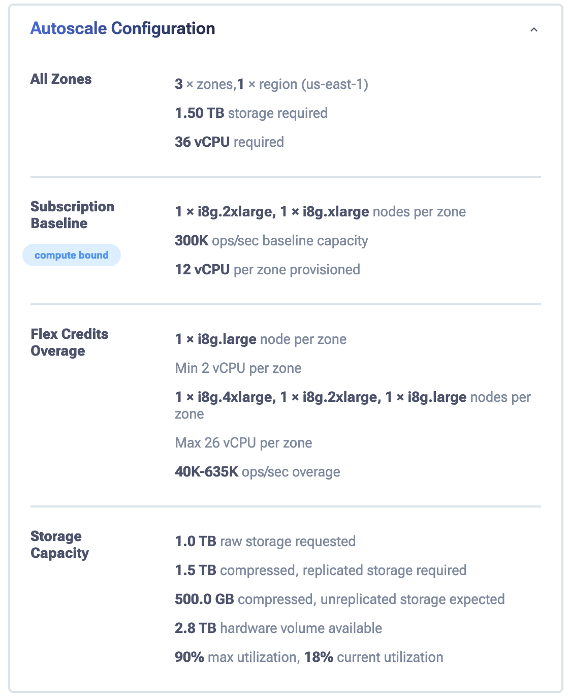
Granularity as a Multiplier
Step size matters. When scaling only happens in large increments, you are forced to round up and overprovision. Mixing node sizes and scaling in smaller increments removes the coarse granularity of uniform nodes and allows much more precise alignment with storage needs.
Targeting 90% storage utilization provides direct, practical control over capacity and cost.
The AI Feature Store example is a clean example with a larger storage footprint (10TB with batch characteristics):

- DynamoDB (provisioned + DAX cache) [$2.2M/year]
- ScyllaDB (hybrid baseline + flex) [$145K/year]
Pay particular attention to the mixed node sizing at the 10 TB mark. Instead of forcing capacity into a single larger step, this configuration uses 1 × i8g.4xlarge, 1 × i8g.2xlarge and 1 × i8g.large per zone. That gets you a 660K ops/sec baseline with 26 vCPUs provisioned per zone.

This matters because the storage fit is much tighter. That’s the real advantage of mixed node sizes: instead of overshooting with coarse, same-size scaling, you can land very close to the intended storage boundary while still meeting baseline performance requirements.
What True Elasticity Means
I keep hearing the same line in database conversations: “We’re elastic.” But many teams still pay for peak capacity 24/7.
I’ve made this mistake myself. You size for the one event you can’t afford to miss, then run underutilized afterward. Six months later, finance is asking questions.
You size for “the event,” the one you can’t afford to miss, then run at a fraction of that capacity post-event. Six months later, Finance is asking questions about your database bill.
Sound familiar? It’s the center of many cost optimization projects; just look at Sharechat’s recent Monster Scale Summit presentation and past blogs about this exact problem.
True elasticity isn’t just scaling infrastructure. It’s aligning billing with workload.
If billing follows demand, elasticity is real.
If billing stays flat, you’re still overprovisioning.
What People Miss About Elasticity
Most people define elasticity as “adding nodes when demand goes up” and then (if you’re doing it well), reducing nodes when the demand drops as well.
That’s only half the job though. True elasticity means you can scale up (or out) quickly, scale down (or in) safely, and keep the same predictable performance while the system rebalances itself in the background.
That last part matters more than people think. In ScyllaDB co-founder Dor Laor’s “holy grail” keynote, one theme he mentioned is that scaling is NOT useful if queries get clobbered while data movement happens. If your P99 latency jumps during the rebalance, then teams using the database naturally lose trust and revert to basic overprovisioning.
No trust in scaling means no true elastic scale. And overprovisioning means just forking out for your worst case scenario 24/7.
Trusting Elastic Scale
While nodes are added and data is streaming, latency still has to remain inside a usable envelope. Dor shared a demo in which the P99 moved from roughly 2.28ms to 2.72ms during scaling – rebalancing in parallel before stabilizing again.
When this is automated (e.g., with ScyllaDB cloud), scaling is blissfully boring, and finance is happier.
Otherwise, scaling is scary, and budgets absorb that fear. (And finance will call, which is even scarier.)
True elastic scale is not about “Can I add capacity?” Hyperscalers have been prefixing the word “elastic” for decades now. True elastic scale is:
- How fast can you add it?
- How safely can you remove it?
- How fine-grained are the increments?
- How stable does latency remain when the topology changes?
- How confidently can your team let the automation run by itself?
If you want to test this with your own use case, start with the scenario browser at calculator.scylladb.com/scenarios
And be sure to try out ScyllaDB X Cloud to see true elastic scale in practice.