Powering a Graph Data System with ScyllaDB + JanusGraph

If you’re reading this blog, you’re probably already aware of the power and speed offered by ScyllaDB. Maybe you’re already using ScyllaDB in production to support high I/O real-time applications. But what happens when you come across a problem that requires some features that aren’t easy to come by with native ScyllaDB?

I’ve recently been working on a Master Data Management (MDM) project with a large cybersecurity company. Their analytics team is looking to deliver a better, faster, and more insightful view of customer and supply chain activity to users around the business.

But anyone who’s tried to build such a solution knows that one of the chief difficulties is encompassing the sheer number and complexity of existing data sources. These data sources often serve as the backends to systems that were designed and implemented independently. Each holds a piece of the overall picture of customer activity. In order to deliver a true solution, we need to be able to bring this disparate data together.

This process requires not just performance and scalability, but also flexibility and the ability to iterate quickly. We seek to surface important relationships, and make them an explicit part of our data model itself.

A graph data system, built with JanusGraph and backed by the power of ScyllaDB, is a great fit for solving this problem.

What is a graph data system?

We’ll break it down into 2 pieces:

• Graph – we’re modeling our data as a graph, with vertices and edges representing each of our entities and relationships
• Data system – we’re going to use several components to build a single system with which to store and retrieve our data

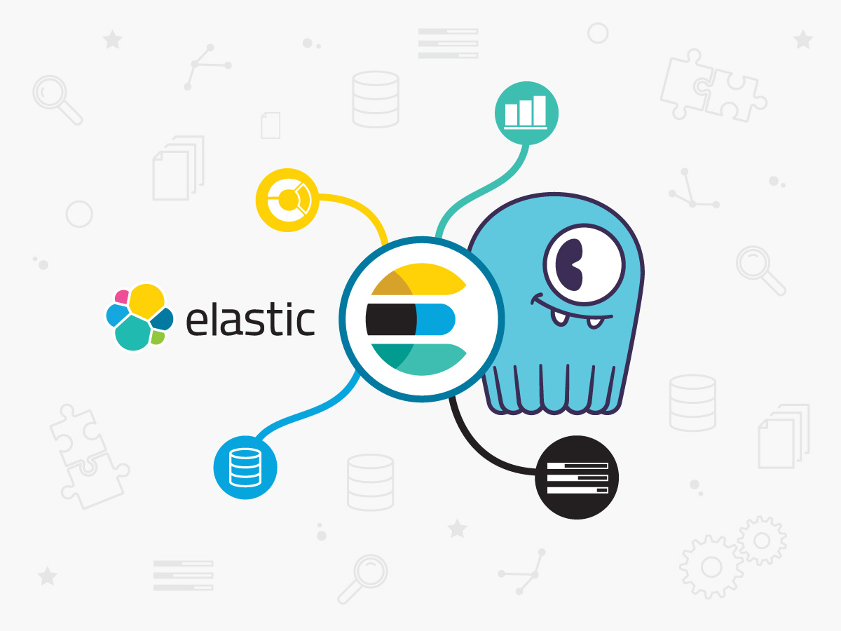
There are several options for graph databases out there on the market, but when we need a combination of scalability, flexibility, and performance, we can look to a system built of JanusGraph, ScyllaDB, and Elasticsearch.

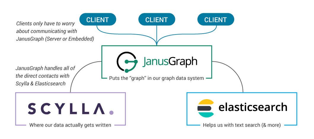
At a high level, here’s how it looks:

Let’s highlight 3 core areas in which this data system really shines:

• Flexibility
• Schema support
• OLTP + OLAP Support

1. Flexibility

While we certainly care about data loading and query performance, the killer feature of a graph data system is flexibility. Most databases lock you into a data model once you’ve started. You define some tables that support your system’s business logic, and then you store and retrieve data from those tables. When you need to add new data sources, deliver a new application feature, or ask innovative questions, you better hope it can be done within the existing schema! If you have to pop the hood on the existing data schema, you’ve begun a time-consuming and error-prone change management process.

Unfortunately, this isn’t the way businesses grow. After all, the most valuable questions to ask today are the ones we didn’t even conceive of yesterday.

Our graph data system, on the other hand, allows us the flexibility to evolve our data model over time. This means that as we learn more about our data, we can iterate on our model to match our understanding, without having to start from scratch. (Check out this article for a more complete walkthrough of the process).

What does this get us in practice? It means we can incorporate fresh data sources as new vertices and edges, without breaking existing workloads on our graph. We can also immediately write query results into our graph — eliminating repetitive OLAP workloads that run daily only to produce the same results. Each new analysis can build on those that came before, giving us a powerful way of sharing production-quality results between teams around the business. All this means that we can answer ever-more insightful questions with our data.

2. Schema Enforcement

While schema-lite may seem nice at first glance, using such a database means that we’re off-loading a lot of work into our application layer. The first- and second-order effects are replicated code across multiple consumer applications, written by different teams in different languages. It’s a huge burden to enforce logic that should really be contained within our database layer.

JanusGraph offers flexible schema support that saves us pain without becoming a hassle. It has solid datatype support out of the box, with which we can pre-define the properties that are possible for a given vertex or edge to contain, without requiring that each vertex must contain all of these defined properties. Likewise, we can define which edge types are allowed to connect a pair of vertices, but this pair of vertices are not automatically forced to have this edge. When we decide to define a new property for an existing vertex, we aren’t forced to write that property for every existing vertex already stored in the graph, but instead can include it only on the applicable vertex insertions.

This method of schema enforcement is immediately beneficial to managing a large dataset – especially one that will be used for MDM workloads. It simplifies testing requirements as our graph sees new use cases, and cleanly separates between data integrity maintenance and business logic.

3. OLTP + OLAP Support

Just like with any data system, we can separate our workloads into 2 categories – transactional and analytical. JanusGraph follows the Apache TinkerPop project’s approach to graph computation. Big picture, our goal is to “traverse” our graph, traveling from vertex to vertex by means of connecting edges. We use the Gremlin graph traversal language to do this. Luckily, we can use the same Gremlin traversal language to write both OLTP and OLAP workloads.

Transactional workloads begin with a small number of vertices (found with the help of an index), and then traverse across a reasonably small number of edges and vertices to return a result or add a new graph element. We can describe these transactional workloads as graph local traversals. Our goal with these traversals is to minimize latency.

Analytical workloads require traversing a substantial portion of the vertices and edges in the graph to find our answer. Many classic analytical graph algorithms fit into this bucket. We can describe these as graph global traversals. Our goal with these traversals is to maximize throughput.

With our JanusGraph – ScyllaDB graph data system, we can blend both capabilities. Backed by the high-IO performance of ScyllaDB, we can achieve scalable, single-digit millisecond response for transactional workloads. We can also leverage Spark to handle large scale analytical workloads.

Deploying our Data System

This is all well and good in theory, so let’s go about actually deploying this graph data system. We’ll walk through a deployment on Google Cloud Platform, but everything described below should be replicable on any platform you choose.

Here’s the design of the graph data system we’ll be deploying:

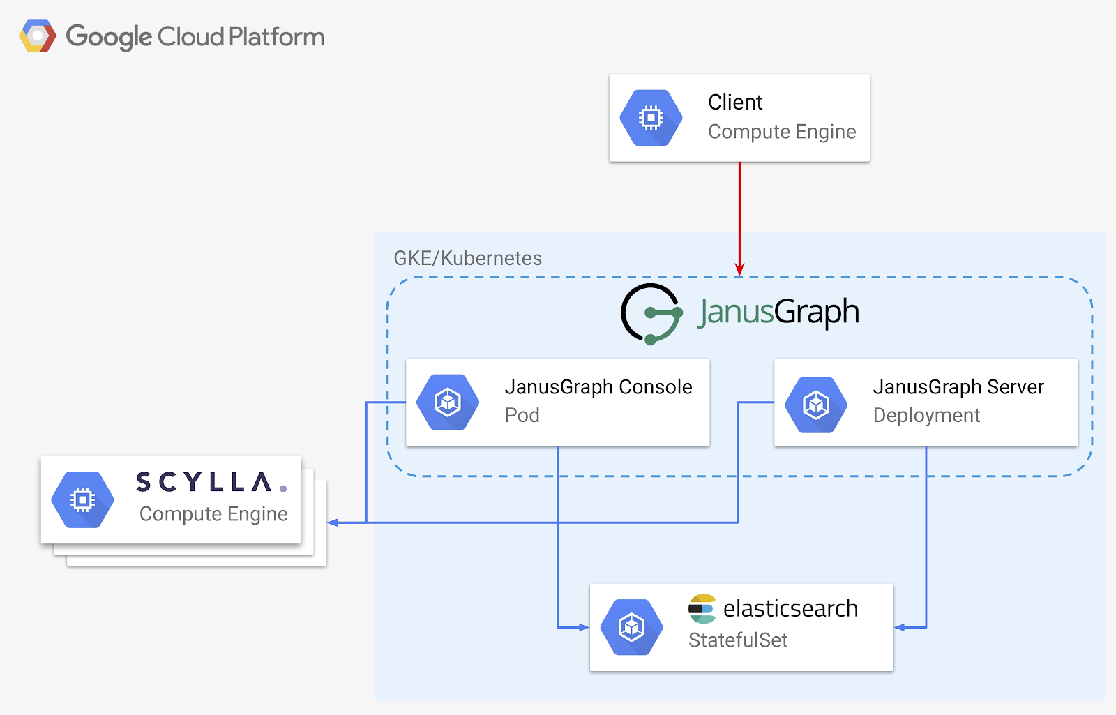
There are three key pieces to our architecture:

• ScyllaDB – our storage backend, the ultimate place where our data gets stored
• Elasticsearch – our index backend, speeding up some searches, and delivering powerful range and fuzzy-match capabilities
• JanusGraph – provides our graph itself, either as a server or embedded in a standalone application

We’ll be using Kubernetes for as much of our deployment as possible. This makes scaling and deployment easy and repeatable regardless of where exactly the deployment is taking place.

Whether we choose to use Kubernetes for ScyllaDB deployment itself depends on how adventurous we are! The ScyllaDB team has been hard at work putting together a production-ready deployment for Kubernetes: ScyllaDB Operator. Currently available as an Alpha release, ScyllaDB Operator follows the CoreOS Kubernetes “Operator” paradigm. While I think this will eventually be a fantastic option for a 100% k8s deployment of JanusGraph, for now we’ll look at a more traditional deployment of ScyllaDB on VMs.

In order to follow along, you can find all of the required setup and load scripts in https://github.com/EnharmonicAI/scylla-janusgraph-examples. You’ll want to change some options as you move to production, but this starting point should demonstrate the concepts and get you moving along quickly.

It’s best to run this deployment from a GCP VM with full access to Google Cloud APIs. You can use one you already have, or create a fresh VM.

gcloud compute instances create deployment-manager \
      --zone us-west1-b \
      --machine-type n1-standard-1 \
      --scopes=https://www.googleapis.com/auth/cloud-platform \
      --image 'centos-7-v20190423' --image-project 'centos-cloud' \
      --boot-disk-size 10 --boot-disk-type "pd-standard"

Then ssh into the VM:

gcloud compute ssh deployment-manager
[ryan@deployment-manager ~]$ ...

We’ll assume everything else is run from this GCP VM. Let’s install some prereqs:

sudo yum install -y bzip2 kubectl docker git
sudo systemctl start docker
curl -O https://repo.anaconda.com/miniconda/Miniconda3-latest-Linux-x86_64.sh
sh Miniconda3-latest-Linux-x86_64.sh

Deploying ScyllaDB

We can use ScyllaDB’s own Google Compute Engine deployment script as a starting point to our ScyllaDB cluster deployment.

git clone https://github.com/scylladb/scylla-code-samples.git
cd scylla-code-samples/gce_deploy_and_install_scylla_cluster

Create a new conda environment and install a few required packages, including Ansible.

conda create --name graphdev python=3.7 -y
conda activate graphdev
pip install ruamel-yaml==0.15.94 ansible==2.7.10 gremlinpython==3.4.0 absl-py==0.7.1

We’ll also do some ssh key housekeeping and apply project-wide metadata, which will simplify connecting to our instances.

touch ~/.ssh/known_hosts
SSH_USERNAME=$(whoami)
KEY_PATH=$HOME/.ssh/id_rsa
ssh-keygen -t rsa -f $KEY_PATH -C $SSH_USERNAME
chmod 400 $KEY_PATH

gcloud compute project-info add-metadata --metadata ssh-keys="$SSH_USERNAME:$(cat $KEY_PATH.pub)"

We’re now ready to setup our cluster. From within the scylla-code-samples/gce_deploy_and_install_scylla_cluster directory we cloned above, we’ll run the gce_deploy_and_install_scylla_cluster.sh script. We’ll be creating a cluster of three ScyllaDB 3.0 nodes, each as an n1-standard-16 VM with 2 NVMe local SSDs.

./gce_deploy_and_install_scylla_cluster.sh \
      -p symphony-graph17038 \
      -z us-west1-b \
      -t n1-standard-4 \
      -n -c2 \
      -v3.0

It will take a few minutes for configuration to complete, but once this is done we can move on to deploying the rest of our JanusGraph components.

Clone the scylla-janusgraph-examples GitHub repo:

git clone https://github.com/EnharmonicAI/scylla-janusgraph-examples
cd scylla-janusgraph-examples

Every command that follows will be run from this top-level directory of the cloned repo.

Setting up a Kubernetes cluster

To keep our deployment flexible and not locked into any cloud provider’s infrastructure, we’ll be deploying everything else via Kubernetes. Google Cloud provides a managed Kubernetes cluster through their Google Kubernetes Engine (GKE) service.

Let’s create a new cluster with enough resources to get started.

gcloud container clusters create graph-deployment \
      --project [MY-PROJECT] \
      --zone us-west1-b \
      --machine-type n1-standard-4 \
      --num-nodes 3 \
      --cluster-version 1.12.7-gke.10 \
      --disk-size=40

We also need to create a firewall rule to allow GKE pods to access other non-GKE VMs.

CLUSTER_NETWORK=$(gcloud container clusters describe graph-deployment \
      --format=get"(network)" --zone us-west1-b)

CLUSTER_IPV4_CIDR=$(gcloud container clusters describe graph-deployment \
      --format=get"(clusterIpv4Cidr)" --zone us-west1-b)

gcloud compute firewall-rules create "graph-deployment-to-all-vms-on-network" \
      --network="$CLUSTER_NETWORK" \
      --source-ranges="$CLUSTER_IPV4_CIDR" \
      --allow=tcp,udp,icmp,esp,ah,sctp

Deploying Elasticsearch

There are a number of ways to deploy Elasticsearch on GCP – we’ll choose to deploy our ES cluster on Kubernetes as a Stateful Set. We’ll start out with a 3 node cluster, with 10 GB of disk available to each node.

kubectl apply -f k8s/elasticsearch/es-storage.yaml
kubectl apply -f k8s/elasticsearch/es-service.yaml
kubectl apply -f k8s/elasticsearch/es-statefulset.yaml

(Thanks to Bayu Aldi Yansyah and his Medium article for laying out this framework for deploying Elasticsearch)

Running Gremlin Console

We now have our storage and indexing backend up and running, so let’s define an initial schema for our graph. An easy way to do this is by launching a console connection to our running ScyllaDB and Elasticsearch clusters.

Build and deploy a JanusGraph docker image to your Google Container Registry.

scripts/setup/build_and_deploy_janusgraph_image.sh -p [MY-PROJECT]

Update the k8s/gremlin-console/janusgraph-gremlin-console.yaml file with your project name to point to your GCR repository image name, and add the correct hostname of one of your ScyllaDB nodes. You’ll notice in the YAML file that we use environment variables to help create a JanusGraph properties file, which we’ll use to instantiate our JanusGraph object in the console with a JanusGraphFactory.

Create and connect to a JanusGraph Gremlin Console:

kubectl create -f k8s/gremlin-console/janusgraph-gremlin-console.yaml
kubectl exec -it janusgraph-gremlin-console -- bin/gremlin.sh

         \,,,/
         (o o)
-----oOOo-(3)-oOOo-----
...
gremlin> graph = JanusGraphFactory.open('/etc/opt/janusgraph/janusgraph.properties')

We can now go ahead and create an initial schema for our graph. We’ll go through this at a high level here, but I walk through a more detailed discussion of the schema creation and management process in this article.

For this example, we’ll look at a sample of Federal Election Commission data on contributions to 2020 presidential campaigns. The sample data has already been parsed and had a bit of cleaning performed on it (shoutout to my brother, Patrick Stauffer, for allowing me to leverage some of his work on this dataset) and is included in the repo as resources/Contributions.csv.

Here’s the start of the schema definition for our contributions dataset:

mgmt = graph.openManagement()

// Define Vertex labels
Candidate = mgmt.makeVertexLabel("Candidate").make()
ename = mgmt.makePropertyKey("name").
    dataType(String.class).cardinality(Cardinality.SINGLE).make()
filerCommitteeIdNumber = mgmt.makePropertyKey("filerCommitteeIdNumber").
    dataType(String.class).cardinality(Cardinality.SINGLE).make()

mgmt.addProperties(Candidate, type, name, filerCommitteeIdNumber)
mgmt.commit()

You can find the complete schema definition code in the scripts/load/define_schema.groovy file in the repository. Simply copy and paste it into the Gremlin Console to execute.

Once our schema has been loaded, we can close our Gremlin Console and delete the pod.

kubectl delete -f k8s/gremlin-console/janusgraph-gremlin-console.yaml

Deploying JanusGraph Server

Finally, let’s deploy JanusGraph as a server, ready to take client requests. We’ll be leveraging JanusGraph’s built-in support for Apache TinkerPop’s Gremlin Server, which means our graph will be accessible to a wide range of client languages, including Python.

Edit the k8s/janusgraph/janusgraph-server-service.yaml file to point to your correct GCR repository image name. Deploying our JanusGraph Server is now as simple as:

kubectl apply -f k8s/janusgraph/janusgraph-server-service.yaml
kubectl apply -f k8s/janusgraph/janusgraph-server.yaml

Loading data

We’ll demonstrate access to our JanusGraph Server deployment by loading some initial data into our graph.

Anytime we load data into any type of database — ScyllaDB, relational, graph, etc — we need to define how our source data will map to the schema that has been defined in the database. For graph, I like to do this with a simple mapping file. An example has been included in the repo, and here’s a small sample:

vertices:
  - vertex_label: Candidate
    lookup_properties:
      FilerCommitteeIdNumber: filerCommitteeIdNumber
    other_properties:
      CandidateName: name
edges:
  - edge_label: CONTRIBUTION_TO
    out_vertex:
      vertex_label: Contribution
      lookup_properties:
        TransactionId: transactionId
    in_vertex:
      vertex_label: Candidate
      lookup_properties:
        FilerCommitteeIdNumber: filerCommitteeIdNumber

This mapping is designed for demonstration purposes, so you may notice that there is repeated data in this mapping definition. This simple mapping structure allows the client to remain relatively “dumb” and not force it to pre-process the mapping file.

Our example repo includes a simple Python script, load_fron_csv.py, that takes a CSV file and a mapping file as input, then loads every row into the graph. It is generalized to take any mapping file and CSV you’d like, but is single-threaded and not built for speed – it’s designed to demonstrate the concepts of data loading from a client.

python scripts/load/load_from_csv.py \
      --data ~/scylla-janusgraph-examples/resources/Contributions.csv \
      --mapping ~/scylla-janusgraph-examples/resources/campaign_mapping.yaml \
      --hostname [MY-JANUSGRAPH-SERVER-LOAD-BALANCER-IP] \
      --row_limit 1000

With that, we have our data system up and running, including defining a data schema and loading some initial records.

Finishing Up

I hope you enjoyed this short foray into a JanusGraph – ScyllaDB graph data system. It should provide you a nice starting point, and demonstrate how easy it is to deploy all the components. Remember to shutdown any cloud resources you don’t want to keep to avoid incurring charges.

We really just scratched the surface of what you can accomplish with this powerful system, and your appetite has been whetted for more. Please send me any thoughts and questions, and I’m looking forward to seeing what you build!