Spark Structured Streaming with ScyllaDB
Hello again! Following up on our previous post on saving data to ScyllaDB, this time, we’ll discuss using Spark Structured Streaming with ScyllaDB and see how streaming workloads can be written in to ScyllaDB. This is the fourth part of our four part series. Make sure you check out all the prior blogs!
Our code samples repository for this post contains an example project along with a docker-compose.yaml file with the necessary infrastructure for running the it. We’re going to use the infrastructure to run the code samples throughout the post and run the project itself, so start it up as follows:
After that is done, launch the Spark shell as in the previous posts:
With that done, let’s get started!
1. Spark Structured Streaming
So far, we’ve discussed datasets in which the entirety of the data was immediately available for processing and that the size of the dataset was known and finite. However, there are many computations that we’d like to perform on datasets of unknown or infinite size. Consider, for example, a Kafka topic to which stock quotes are continuously written:
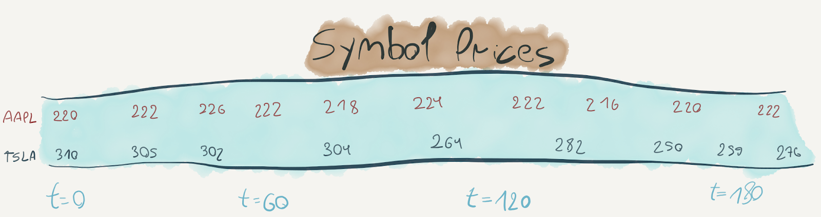
We might want to keep track of the hourly range of change in the symbol’s price, like so:
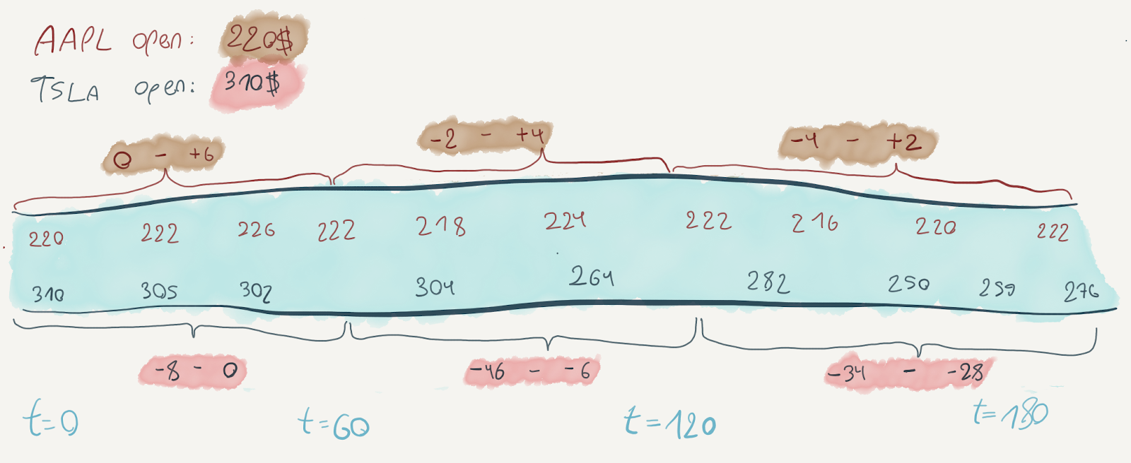
The essence of this computation is to continuously compute the minimum and maximum price values for the symbol in every hour, and when the hour ends – output the resulting range. To do this, we must be able to perform the computation incrementally as the data itself would arrive incrementally.
Streams, infinite streams in particular, are an excellent abstraction for performing these computations. Spark’s Structured Streaming module can represent streams as the same dataframes we’ve worked with. Many transformations done on static dataframes can be equally performed on streaming dataframes. Aggregations like the one we described work somewhat differently, and require a notion of windowing. See the Spark documentation for more information on this subject.
The example project we’ve prepared for this post uses Spark Structured Streaming, ScyllaDB and Kafka to create a microservice for summarizing daily statistics on stock data. We’ll use this project to see how streams can be used in Spark, how ScyllaDB can be used with Spark’s streams and how to use another interesting ScyllaDB feature – materialized views. More on that later on!
The purpose of the service is to continuously gather quotes for configured stocks and provide an HTTP interface for computing the following 2 daily statistics:
- The difference between the stock’s previous close and the stock’s maximum price in the day;
- The difference between the stock’s previous close and the stock’s minimum price in the day.
Here’s an example of the output we eventually expect to see from the service:
To get things going, run the two scripts included in the project:
These will create the ScyllaDB schema components and start the Spark job. We’ll discuss the ScyllaDB schema shortly; first, let’s see what components do we have for the Spark job.
NOTE: The service polls live stock data from a US-based exchange. This means that if you’re outside trading hours (9:30am – 4pm EST), you won’t see data in ScyllaDB changing too much.
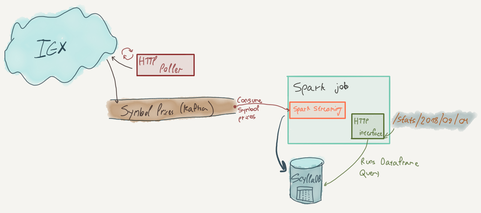
There are 3 components to our service:
- An Akka Streams-based graph that continuously polls IEX for stock data quotes, and writes those quotes to a Kafka topic. Akka Streams is a toolkit for performing local streaming computations (compared to Spark which performs distributed streaming computations). We’ll discuss it shortly and won’t delve too much into its details. If you’re interested, check out the docs – Akka Streams is an extremely expressive library and can be very useful on the JVM.
- A Spark Streaming based component that creates a DataFrame from the stock quotes topic, extracts relevant fields from the entries and writes them to ScyllaDB.
- An HTTP interface that runs a regular Spark query against ScyllaDB to extract statistics.
For starters, let’s see the structure of our input data. Here’s an abridged JSON response from IEX’s batch quote API:
Our polling component will transform the entries in the response to individual messages sent to a Kafka topic. Each message will have a key equal to the symbol, a timestamp equal to the latestUpdate value and a value equal to the value of the quote JSON.
Next, our Spark Streaming component will consume the Kafka topic using a streaming query. This is where things get more interesting, so let’s fiddle with some streaming queries in the Spark shell. Here’s a query that will consume the quotes Kafka topic and print the consumed messages as a textual table:
If the quotes application is running properly, this query should continuously print the data it has been writing to the Kafka topic as a textual table:
Every row passing through the stream is a message from Kafka; the row’s schema contains all the data and metadata for the Kafka messages (keys, values, offsets, timestamps, etc.). The textual tables will keep appearing until you stop the query. It can get a bit spammy, So let’s stop it:
The type of query is StreamingQuery – a handle to a streaming query running in the background. Since these queries are meant to be long-running, it is important to be able to manage their lifecycle. You could, for example, hook up the StreamingQuery handle to an HTTP API and use the query.status method to retrieve a short description of the streaming query’s status:
In any case, the schema for the streaming query is not suitable for processing – the messages are in a binary format. To adapt the schema, we use the DataFrame API:
This should print out a table similar to this:
That looks better – the key for each Kafka message is the symbol and the body is the quote data from IEX. Let’s stop the query and figure out how to parse the JSON.
This would be a good time to discuss the schema for our ScyllaDB table. Here’s the CREATE TABLE definition:
It’s pretty straightforward – we keep everything we need to calculate the difference from the previous close for a given symbol at a given timestamp. The partitioning key is the symbol, and the clustering key is the timestamp. This primary key is not yet suitable for aggregating and extracting the minimum and maximum differences of all symbols for a given day, but we’ll get there in the next section.
To parse the JSON from Kafka, we can use the from_json function defined in org.apache.spark.sql.functions. This function will parse a String column to a composite data type given a Spark SQL schema. Here’s our schema:
The schema must be defined up front in order to properly analyze and validate the entire streaming query. Otherwise, when we subsequently reference fields from the JSON, Spark won’t know if these are valid references or not. Next, we modify the streaming query to use that schema and parse the JSON:
Now that it’s parsed, we can extract the fields we’re interested in to create a row with all the data we need at the top level. We’ll also cast the timestamp to a DataType and back in order to truncate it to the start of the day:
This should print out a table similar to this, which is exactly what we want to write to ScyllaDB:
2. Writing to ScyllaDB using a custom Sink
Writing to ScyllaDB from a Spark Structured Streaming query is currently not supported out of the box with the Datastax connector (tracked by this ticket). Luckily, implementing a simplistic solution is fairly straightforward. In the sample project, you will find two classes that implement this functionality: ScyllaDBSinkProvider and ScyllaDBSink.
ScyllaDBSinkProvider is a factory class that will create instances of the sink using the parameters provided by the API. The sink itself is implemented using the non-streaming writing functionality we’ve seen in the previous article. It’s so short we could fit it entirely here:
This sink will write any incoming DataFrame to ScyllaDB, assuming that the connector has been configured correctly. This interface is indicative of the way Spark’s streaming facilities operate. The streaming query processes the incoming data in batches; it’ll create batches by polling the source for data in configurable intervals. Whenever a DataFrame for a batch is created, tasks for processing the batch will be scheduled on the cluster.
To integrate this sink into our streaming query, we will replace the argument to format after writeStream with the full name of our provider class. Here’s the full snippet; there’s no need to run it in the Spark shell, as it is what the quotes service is running:
We’re also specifying an output mode, which is required by Spark (even though our sink will ignore it), parameters for the sink and the checkpoint location. Checkpoints are Spark’s mechanism for storing the streaming query’s state and allowing it to resume later. A detailed discussion is beyond the scope of this article; Yuval Itzchakov has an excellent post with more details on checkpointing if you’re interested.
Once that streaming query is running, Spark will write each DataFrame (which corresponds to a batch produced by reading from Kafka) to ScyllaDB using our sink. We’re done with this component; let’s see how we’re going to serve our statistics over HTTP by querying ScyllaDB.
3. Serving the statistics from ScyllaDB
As it stands, our ScyllaDB table stores the data queried from IEX with a partition key of symbol and a clustering key of timestamp. This is good for handling queries that deal with a single symbol; ScyllaDB would only need to visit a single partition when processing them. However, the statistics we’d like to compute are the min/max change in price for all symbols in a given day. Therefore, to efficiently handle those queries, the primary key needs to be adjusted.
What options do we have? The easiest one is to just store the data differently. We could modify our schema to use a primary key of ((day), symbol, timestamp). This way, the statistics could be computed by visiting only one partition. However, when we would like to answer queries that focus on a single symbol, we’ll end up with the same problem.
To solve this problem, we’ll use an interesting feature offered by ScyllaDB: materialized views. If you’re familiar with materialized views from relational databases, the ScyllaDB implementation shares the name but is much more restrictive to maintain efficiency. See these articles for more details.
We will create a materialized view that will repartition the original data using the optimal primary key for our queries; here’s the CQL statement included in the create-tables.sh script:
The materialized view will be maintained by ScyllaDB and will update automatically whenever we update the quotes table. We can now query it as an ordinary table. We will perform the aggregations in Spark using a plain DataFrame query:
This query, included in the HTTP routes component, aggregates the data for September 20th by symbol and computes the minimum and maximum prices for the symbols. These are then used to compute the minimum and maximum change in price compared to the previous close.
Whenever an HTTP request is sent to the service, this query is run with different date parameters and the results are sent over the HTTP response.
4. Summary
This post contained a (very) short introduction to streaming computations in general, streaming computations with Spark Structured Streaming and writing to ScyllaDB from Spark Structured Streaming. Now, streaming is a vast subject with many aspects and nuances – state and checkpointing, windowing and high watermarks, and so forth. To learn more about the subject, I recommend two resources:
- Streaming Systems, by Tyler Akidau et al. – an excellent book that comprehensively covers everything related to streams, from authors that basically invented the subject;
- The Structured Streaming programming guide – a great overview of the module and its capabilities.
We’ve also covered the use of ScyllaDB’s materialized views – a very useful feature for situations where we need to answer a query that our schema isn’t built to handle.
Thanks for reading, and stay tuned for our next article, in which we will discuss the ScyllaDB Migrator project.