

ScyllaDB powers real-time AI with low latency, high throughput, and billion-scale data.
Learn MoreScyllaDB powers real-time AI with low latency, high throughput, and billion-scale data.
Learn More
ScyllaDB is purpose-built for data-intensive apps that require high throughput & predictable low latency.
Learn More
ScyllaDB Cloud and Google Cloud Bigtable are both hosted NoSQL, wide-column databases. Google Cloud Bigtable, the commercially available version of Bigtable, is the database used internally at Google to power many of its apps and services.
In this Bigtable performance benchmark, we will simulate a scenario in which the user has a predetermined workload with the following SLA: 90,000 operations per second (ops), half of those being reads and half being updates, and the need to survive zone failures. We set business requirements so that 95% of the reads must be completed in 10ms or less and will determine the minimum cost of running such a cluster in each of the offerings. We will show that ScyllaDB Cloud accomplishes this at one-third the cost of Cloud Bigtable pricing.
ScyllaDB is a drop-in-replacement for Cassandra and DynamoDB. Cassandra, in turn, was inspired by the original Bigtable and Dynamo papers. Cassandra is often described as the “daughter” of Dynamo and Bigtable. Thus, Scylla and Bigtable share the same family tree. Given their architectural similarities and differences, it’s critical for IT teams to understand the relative performance characteristics of each database and choose from the best Bigtable alternatives.
The following Scylla Cloud vs Google Cloud Bigtable benchmark tests demonstrate that ScyllaDB Cloud performs 26X better than Google Cloud Bigtable when applied with real-world, unoptimized data distribution. ScyllaDB maintains target SLAs, while Cloud Bigtable fails to do so. Finally, we investigate the worst case for both offerings, where a single hot row is queried. While both databases fail to meet the 90,000 ops SLA, ScyllaDB processes 195x more requests than Cloud Bigtable processing.
The goal of this ScyllaDB vs Bigtable benchmark was to perform 90,000 operations per second in the cluster (50% updates, 50% reads) while keeping read latencies at 10ms or lower for 95% of the requests.
The cluster runs in three different zones, to provide high availability and lower local latencies. This is important not only to protect against entire-zone failures, which are rare, but also to reduce latency spikes and timeouts of Cloud Bigtable. Zone maintenance jobs can impact Cloud Bigtable latencies. (For reference, see this article).
Increasing the Cloud Bigtable replication factor means adding replication clusters. Cloud Bigtable claims that each group node (per replica cluster) should be able to perform 10,000 operations per second at 6ms latencies, although it does not specify at which percentile. It also makes the disclaimer that those numbers are workload-dependent. Still, we use them as a basis for analysis and will start our tests by provisioning three clusters of 9 nodes each. We will then increase the total size of the deployment by adding a node to each cluster until the desired SLAs are met.
For ScyllaDB, we selected a 3-node cluster of AWS i3.4xlarge instances. The selection is based on ScyllaDB’s recommendation of leaving 50% free space per instance and the fact that this is the smallest instance capable of holding the data generated in the population phase of the benchmark— each i3.4xlarge can store a total of 3.8TB of data and should be able to comfortably hold 1TB at 50% utilization. We will follow the same procedure as Cloud Bigtable and keep adding nodes (one per zone) until our SLA is met.
In GCP Bigtable terminology, replication is achieved by adding additional clusters in different zones. To withstand the loss of two of them, we set three replicas, as shown below in Figure 1:
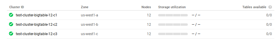
Figure 1: Example setting of Google Cloud Bigtable in three zones. A single zone is enough to guarantee that node failures will not lead to data loss, but is not enough to guarantee service availability/data-survivability if the zone is down.
Cloud Bigtable allows for different consistency models as described in their documentation according to the cluster routing-model. By default, data will be eventually consistent and multi-cluster routing is used, which makes for the highest availability of data. Since eventual consistency is our goal, Cloud Bigtable has their settings kept at the defaults and multi-cluster routing is used. Figure 2 shows the explanation about routing that can be seen in Cloud Bigtable’s routing selection interface.

Figure 2: Google Cloud Bigtable settings for availability. In this test, we want to guarantee maximum availability across three zones.
We verified that the cluster is, indeed, set up in this mode, as it can be seen in Figure 3 below:
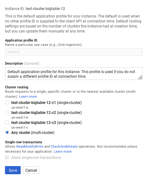
Figure 3: Google Cloud Bigtable is configured in multi-cluster mode.
For ScyllaDB, consistency is set in a per-request basis and is not a cluster-wide property, as described in ScyllaDB’s documentation (referred to as “tunable consistency”). Unlike Cloud Bigtable, in ScyllaDB’s terminology all nodes are part of the same cluster. Replication across availability zones is achieved by adding nodes present in different racks and setting the ScyllaDB replication factor to match. We set up the ScyllaDB Cluster in a single datacenter (us-east-1), and set the number of replicas to three (RF 3), placing them in three different availability zones within the us-east-1 region for AWS. This setup can be seen in Figure 4 below:
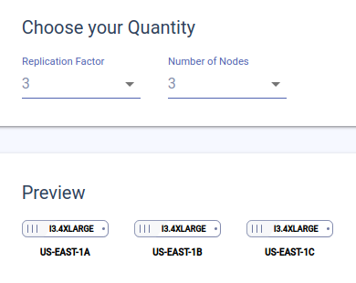
Figure 4: ScyllaDB Cloud will be set up in 3 availability zones. To guarantee data durability, ScyllaDB Cloud requires replicas, but that also means that any ScyllaDB Cloud setup is able to maintain availability of service when availability zones go down.
Eventual consistency is achieved by setting the consistency of the requests to LOCAL_ONE for both reads and writes. This will cause ScyllaDB to acknowledge write requests as successful when one of the replicas respond, and serve reads from a single replica. Mechanisms such as hinted handoff and periodic repairs are used to guarantee that data will eventually be consistent among all replicas.
We used the YCSB benchmark running across multiple zones in the same region as the cluster. To achieve the desired distribution of 50% reads and 50% updates, we will use YCSB’s Workload A, which is already pre-configured to have that ratio. We will keep the workload’s default record size (1kB), and add one billion records— enough to generate approximately 1TB of data on each database.
We then ran the load for the total time of 1.5 hours. At the end of the run, YCSB produces a latency report that includes the 95th-percentile latency per client. Aggregating percentiles is a challenge on its own. Throughout this report, we will use the client that reported the highest 95th-percentile as our number. While we understand this is not the “real” 95th-percentile of the distribution, it at least maps well to a real-world situation where the clients are independent and we want to guarantee that no client sees a percentile higher than the desired SLA.
We will start the SLA investigation by using a uniform distribution, since this guarantees good data distribution across all processing units of each database while being adversarial to caching. This allows us to make sure that both databases are exercising their I/O subsystems and not relying only on in-memory behavior.
Our instance has 3 clusters all in the same region. We spawned 12 small (4 cpus, 8GB RAM) GCE machines, 4 in each of the 3 zones where Cloud Bigtable clusters are located. Each client ran 1 YCSB client with 50 threads and a target of 7,500 ops per second; for a total of 90,000 operations per second. The command used is:
~/YCSB/bin/ycsb run googlebigtable -p requestdistribution=uniform -p columnfamily=cf -p google.bigtable.project.id=$PROJECT_ID -p google.bigtable.instance.id=$INSTANCE_ID -p google.bigtable.auth.json.keyfile=auth.json -p recordcount=1000000000 -p operationcount=125000000 -p maxexecutiontime=5400 -s -P ~/YCSB/workloads/$WORKLOAD -threads 50
Our ScyllaDB cluster has 3 nodes spread across 3 different Availability Zones. We spawned 12 c5.xlarge machines, 4 in each AZ, running one YCSB client with 50 threads and a target of 7,500 ops per second; for a total of 90,000 ops per second. For this benchmark, we used a YCSB version that handles prepared statements, which means all queries will be compiled only once and then reused. We also used the ScyllaDB-optimized Java driver. Although ScyllaDB is compatible with Apache Cassandra drivers, it ships with optimized drivers that increase performance through ScyllaDB-specific features.
~/YCSB/bin/ycsb run cassandra-cql -p hosts=$HOSTS -p recordcount=1000000000 -p operationcount=125000000 -p requestdistribution=uniform -p cassandra.writeconsistencylevel=LOCAL_ONE -p cassandra.readconsistencylevel=LOCAL_ONE -p maxexecutiontime=5400 -s -P workloads/$WORKLOAD -threads 50 -target 750
The results are summarized in Table 1. Cloud Bigtable is unable to meet the target of 90,000 operations per second with the initial setup of 9 nodes per cluster. We report the latencies for completeness, but they are not relevant since the cluster was clearly at a bottleneck and operating over capacity. During this run, we can verify that this is indeed the case by looking at Cloud Bigtable’s monitoring dashboard. Figure 4 shows the average CPU utilization among the nodes, already way above the recommended threshold of 70%. Figure 5 shows CPU utilization at the hottest node: for those, we are already at the limit.
GCP Bigtable is still unable to meet the desired amount of operations with clusters of 10 nodes, and is finally able to do so with 11 nodes. However, the 95th percentile for reads is above the desired goal of 10 ms so we take an extra step in expanding the clusters. With clusters of 12 nodes each, Cloud Bigtable is finally able to achieve the desired SLA.
ScyllaDB Cloud had no issues meeting the SLA at its first attempt.
The above was actually a fast-forward version of what we encountered. Originally, we didn’t start with the perfect uniform distribution and chose the real-life-like Zipfian distribution. Over and over we received only 3,000 operations per second instead of the desired 90,000. We thought something was wrong with the test until we cross-checked everything and switched to uniform distribution testing. Since Zipfian test results mimic real-life behaviour, we ran additional tests and received the same original poor result (as described in the Zipfian section below).
For uniform distribution, the results are shown in Table 1, and the average and hottest node CPU utilizations are shown just below in Figures 5 and 6, respectively.
| OPS | Maximum Latency P95 (microseconds) | Cost per replica/AZ per year ($USD) | Total Cost for 3 replicas/AZ per year ($USD) | ||
| READ | UPDATE | ||||
| Cloud Bigtable 3×9 nodes (27 nodes) | 79,890 | 27,679 | 27,183 | $53,334.98 | $160,004.88 |
| Cloud Bigtable 3×10 nodes (30 nodes) | 87,722 | 21,199 | 21,423 | $59,028.96 | $177,086.88 |
| Cloud Bigtable 3×11 nodes (33 nodes) | 90,000 | 12,847 | 12,479 | $64,772.96 | $184,168.88 |
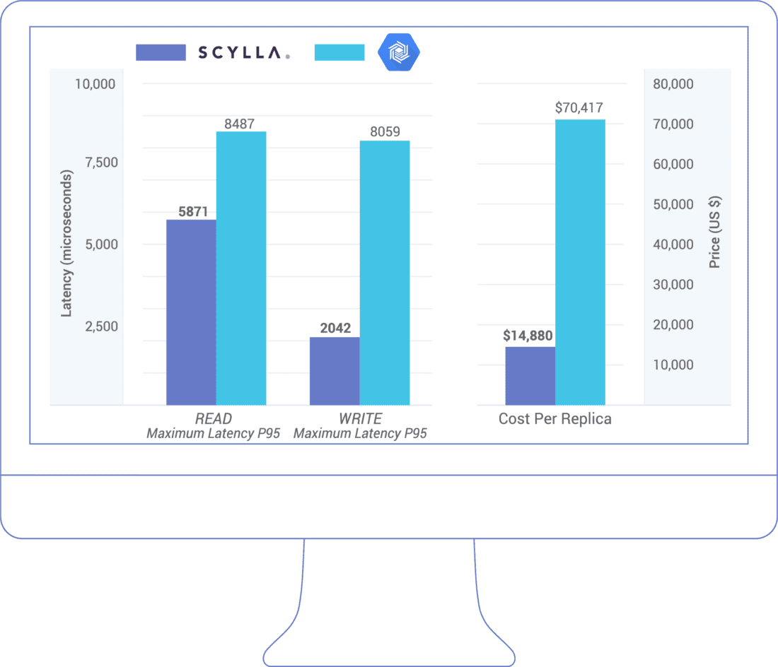
| Cloud Bigtable 3×12 nodes ( 36 nodes) | 90,000 | 8,487 | 8,059 | $70,416.96 | $211,250.88 |
| ScyllaDB 3×1 nodes ( 3 nodes) | 90,000 | 5,871 | 2,042 | $14,880 | $44,680 |
Table 1: ScyllaDB Cloud is able to meet the target SLA with just one instance per zone (for a total of three). 12 Cloud Bigtable instances per cluster (total of 36) are required to meet the performance characteristics of the benchmark workload. For both ScyllaDB Cloud and Cloud Bigtable, costs exclude network transfers. Cloud Bigtable price was obtained from Google Calculator and used as-is, and for ScyllaDB Cloud prices were obtained from the official pricing page, with the network and backup rates subtracted. For ScyllaDB Cloud, the price doesn’t vary with the amount of data stored up to the instance’s limit. For Cloud Bigtable, price depends on data that is actually stored up until the instance’s maximum. We use 1TB in the calculations in this table.
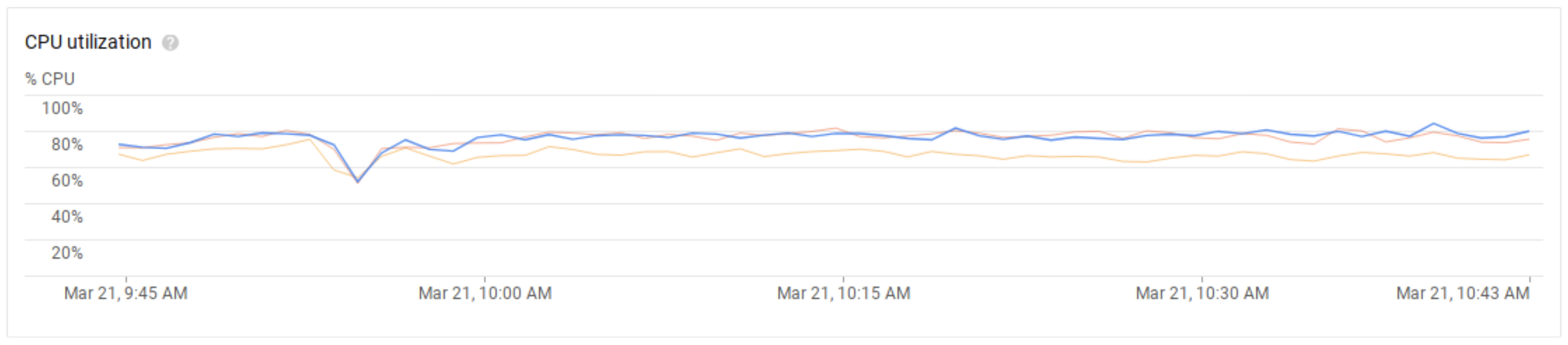
Figure 5: Average CPU load on a 3-cluster 9-node Cloud Bigtable instance, running Workload A
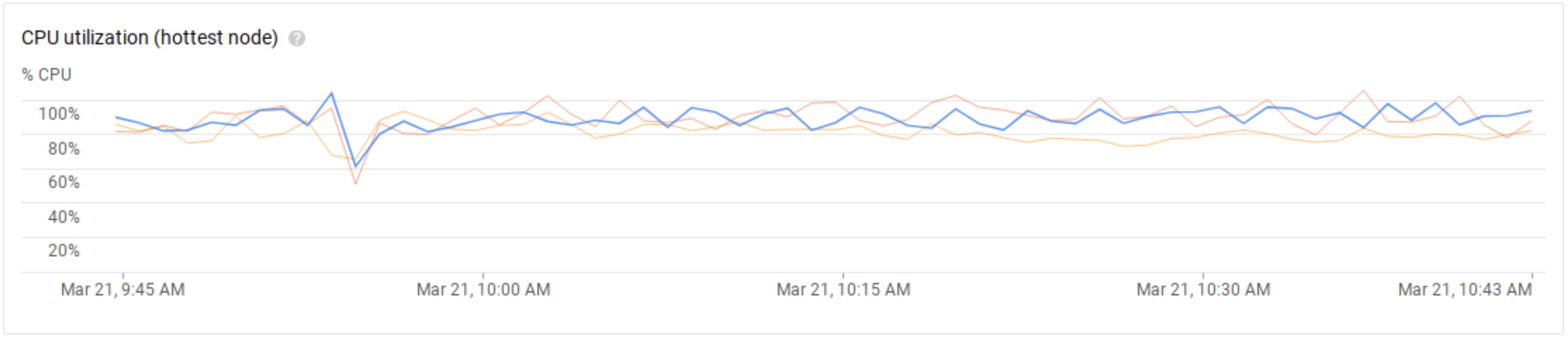
Figure 6: Hottest node CPU load on a 3-cluster 9-node Cloud Bigtable instance, running Workload A
ScyllaDB Cloud and Cloud Bigtable both behave better under uniform data and request distribution; all users are advised to strive for that. No matter how much work goes into good partitioning, workloads in real life often behave differently — either continuously due to some unexpected systemic issue or temporarily due to a change in access patterns. That affects performance in practice.
For example, a user profile application can see patterns in time where groups of users are more active than others. An IoT application tracking data for sensors can have sensors that end up accumulating more data than others, or having time periods in which data gets clustered. A famous case is “the dress that broke the internet,” where a lively discussion among tens of millions of Internet users about the color of a particular dress led to issues in handling traffic for the underlying database.
In this session we will keep the cluster size determined in the previous phase constant, and study how both offerings behave under such scenarios.
To simulate real-world conditions, we changed the request distribution in the YCSB loaders to a Zipfian distribution. We have kept all other parameters the same, so the loaders are still trying to send the same 90,000 requests per second (with 50% reads, 50% updates).
Zipfian distribution was originally used to describe word frequency in languages. However, this distribution curve, known as Zipf’s Law, has also shown correlation to many other real-life scenarios. It can often indicate a form of “rich-get-richer” self-reinforcing algorithm, such as a bandwagon or network effect, where the distribution of results is heavily skewed and disproportionately weighted.
For instance, in searching over time, once a certain search result becomes popular, more people click on it, and thus, it becomes an increasingly popular search result. Examples include the number of “likes” different NBA teams have on social media, as shown in Figure 7, or the activity distribution among users of the Quora website.
When these sort of result skews occur in a database, it can lead to incredibly unequal access to the database and, resultantly, poor performance. For database testing, this means we’ll have keys randomly accessed in a heavy-focused distribution pattern that allows us to visualize how the database in question handles hotspot scenarios.
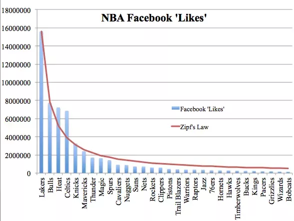
Figure 7: The number of “likes” NBA teams get on Facebook follows a Zipfian distribution.
The results of our Zipfian distribution test are summarized in Table 2. Cloud Bigtable is not able to sustain 90,000 requests per second. It can process only 3,450 requests per second. ScyllaDB Cloud, on the other hand, actually gets slightly better in its latencies. This result is surprising at first until you realize the more you hit the same hot partitions, the more hits will be made against ScyllaDB’s unified cache.
| Zipfian Distribution | |||
| Overall Throughput (ops/second) | p95 latency, milliseconds | ||
| READ | UPDATE | ||
| Cloud Bigtable 3×10 nodes (30 nodes) | 3,450 | 1,601 ms | 122 ms |
| ScyllaDB Cloud | 90,000 | 3 ms | 1 ms |
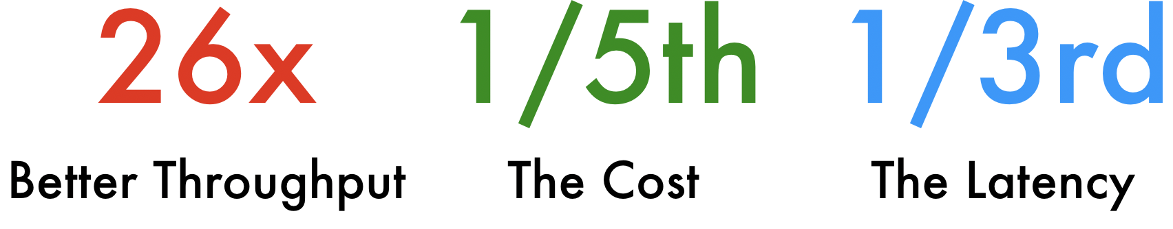
Table 2: Results of ScyllaDB Cloud vsCloud Bigtable under the Zipfian distribution. Cloud Bigtable is not able to sustain the full 90,000 requests per second. ScyllaDB Cloud was able to sustain 26x the throughput, and with read latencies 1/800th and write latencies less than 1/100th of Cloud Bigtable.
Cloud Bigtable can serve only 180 requests per second and then latencies shoot up. Figure 8, below, demonstrates how the hottest node is bottlenecked, although the overall CPU utilization is low.
The benchmark was not run to determine how many Cloud Bigtable nodes would be needed to achieve the same required 90,000 ops/second throughput under Zipfian distribution. Cloud Bigtable’s throughput under Zipfian distribution was 1/26th that of ScyllaDB.
Assuming that the Bigtable database scales linearly under a Zipfian distribution scenario, it would need over 300 nodes (as a single replica/AZ) to more than 900 nodes (triple replicated) to achieve the 90,000 ops required by the SLA. The annual cost for a single-replicated cluster of that scale would have been approximately $1.8 million annually; or nearly $5.5 million if triple-replicated.
That would be 41x or 123x the cost of ScyllaDB, respectively. Assuming a middle-ground situation in which Cloud Bigtable was deployed in two availability zones, the cost would be approximately $3.6 million annually; 82x the cost of ScyllaDB Cloud running triple-replicated.
These are only hypothetical projections and welcome others to run these Zipfian tests themselves to see how many nodes would be required to meet the 90,000 ops/second test requirement on Cloud Bigtable.
How does ScyllaDB vs BigTable performance compare in the extreme case of a single hot row that’s accessed over a time interval? Keeping the same YCSB parameters, the client submits 90,000 requests per second, but sets the key population of the workload to a single row. Results are summarized in Table 2.
| Single Hot Row | |||
| Overall Throughput (ops/second) | p95 latency, milliseconds | ||
| READ | UPDATE | ||
| Cloud Bigtable 3×10 nodes (30 nodes) | 180 | 7,733 ms | 5,365 ms |
| ScyllaDB Cloud | 35,400 | 73 ms | 13 ms |
Table 3: ScyllaDB Cloud and Cloud Bigtable results when accessing a single hot row. Both databases see their throughput reduced for this worst-case scenario, but ScyllaDB Cloud is still able to achieve 35,400 requests per second. Given the data anomaly, neither ScyllaDB Cloud nor Cloud Bigtable were able to meet the SLA, but ScyllaDB was able to perform much better, with nearly 200 times Cloud Bigtable’s anemic throughput and multi-second latency. This ScyllaDB environment is 1/5th the cost of Cloud Bigtable.
Cloud Bigtable can serve only 180 requests per second and then latencies shoot up. Figure 8, below, demonstrates how the hottest node is bottlenecked, although the overall CPU utilization is low.
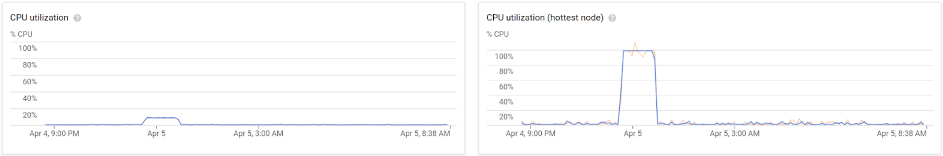
Figure 8: While handling a single hot row, Cloud Bigtable shows its hottest node at 100% utilization even though overall utilization is low.
While ScyllaDB Cloud is also unable to keep up with client requests at the desired throughput, the rate drops to a baseline of 35,400 requests per second — 196 times Cloud Bigtable throughput . While higher throughput can always be achieved by increasing concurrency, such concurrency comes with a fiscal cost, and it would also have the negative side-effect of worsening latencies. A more efficient engine, such as ScyllaDB, guarantees better behavior during worst-case scenarios.
The results for both the Zipfian and Single Hot Row scenario clearly demonstrate that ScyllaDB Cloud performs better under real-world conditions than Cloud Bigtable.
When both ScyllaDB Cloud and Google Cloud Bigtable are exposed to synthetic lab, well-behaved, uniform workload, ScyllaDB Cloud is 1/5th the cost of Cloud Bigtable. However, under more likely real-world Zipfian distribution of data, which we see in both our own customer experience as well as academic research and empirical validation, Cloud Bigtable performance was nowhere near meeting the desired SLA and is therefore not practical.
To recap our results, as shown below, ScyllaDB Cloud is 1/5th the expense while providing 26x the performance of Cloud Bigtable, better latency and better behavior in the face of hot rows. ScyllaDB met its SLA with 90,000 OPS and low latency response times while Cloud Bigtable couldn’t do more than 3,450 OPS. As an exercise to the reader, try to execute or compute the total cost of ownership of a Cloud Bigtable, real-life workload at 90,000 OPS. Would it be 5x (the ScyllaDB savings) multiplied by 26x? Even if you decrease the Bigtable replication to two zones or even a single zone, the difference is enormous.
As you can see, ScyllaDB has a notable advantage on every metric and on through data test we conducted. We invite you to judge how much better it is in a scenario similar to your needs.
Furthermore, Cloud Bigtable is an offering available exclusively on the Google Cloud Platform (GCP), which locks the user in to Google as both the database provider and infrastructure service provider — in this case, to its own public cloud offering.
ScyllaDB Cloud is a managed offering of the ScyllaDB Enterprise database. It is available on Amazon Web Services (AWS), and will soon be available on GCP and other public clouds. Beyond ScyllaDB Cloud, ScyllaDB also offers Open Source and Enterprise versions, which can be deployed to private clouds, on-premises, or co-location environments. While ScyllaDB Cloud is ScyllaDB’s own public cloud offering, ScyllaDB provides greater flexibility and does not lock-in users to any particular deployment option.
Yet while vendors like us can make claims, the best judge of performance is your own assessment based on your specific use case. Give us a try on ScyllaDB Cloud and please feel free to drop in to ask questions via our Slack channel.
Getting started takes only a few minutes. ScyllaDB has an installer for every major platform. If you get stuck, we’re here to help.