Watching ScyllaDB serving 1 Million operations per second

In this post we present more details about ScyllaDB’s behavior during the benchmark behind these results.

ScyllaDB is all about performance and thus we decided to push metrics using collectd protocol.We sprinkled quite a few counters, which can be used to monitor its internals. ScyllaDB can be configured to export them periodically to collectd. In our setup collectd was configured to further sent the events to riemann. and riemann-dash was used to monitor it.

As explained in the architecture section, ScyllaDB server is composed out of many shards as the number of cores. Those shards are internal objects, transparent for client-side tools. A shard is self-contained resource unit and owns a single cpu (thread), ram (NUMA local), own sstables and even its own NIC queue. The magic behind ScyllaDB is to activate all shards in parallel, where the load distributed evenly over all shards.

ScyllaDB counters used in this post are:

• transport-<shard>/total_requests-requests_served – the number of CQL requests served per time unit
• cache-<shard>/bytes-total – memory reserved for cache
• cache-<shard>/bytes-used – memory used by live objects inside cache
• cache-<shard>/total_operations-hits – number of cache hits per time unit
• cache-<shard>/total_operations-misses – number of cache misses per time unit
• cache-<shard>/total_operations-insertions – number of entries inserted into cache per time unit
• cache-<shard>/total_operations-merges – number of entries merged into cache per time unit
• cache-<shard>/objects-partitions – number of partitions held by cache
• lsa-<shard>/bytes-non_lsa_used_space – memory allocated using standard allocator
• lsa-<shard>/bytes-total_space – memory reserved for log-structured allocator (LSA)
• lsa-<shard>/bytes-used_space – memory used by live objects inside LSA

Each shard exports its own value of the counters (hence the <shard> part). To see a grand total for all shard, we can define a new aggregate event in Riemann config. For example, this is how transport/total_requests_served is defined:

    (where (service #"transport.*requests_served")
        (coalesce (smap folds/sum
        (with {:service "transport/total_requests_served"} index)))
    )

In addition to ScyllaDB counters, it’s worthwhile to monitor statistics of disk and network interface:

• interface-<name>/if_packets/rx
• interface-<name>/if_packets/tx
• interface-<name>/if_octets/rx
• interface-<name>/if_octets/tx
• disk-<name>/disk_octets/read
• disk-<name>/disk_octets/write

Those are exported by standard collectd plugins.

Populating the database

ScyllaDB doesn’t depend on the system’s page cache for caching sstable data. Instead, it takes over the memory which in case of Cassandra would be dedicated for page cache and manages it on its own. We can monitor cache performance using counters, which will be demonstrated below.

ScyllaDB uses two memory allocators. One is the Seastar allocator, which is used for general purpose allocations. The other one is the log-structured allocator (LSA) which is used to allocate objects belonging to both memtable and cache.

Below is a screenshot of a dashboard when the database is populated with new partitions:

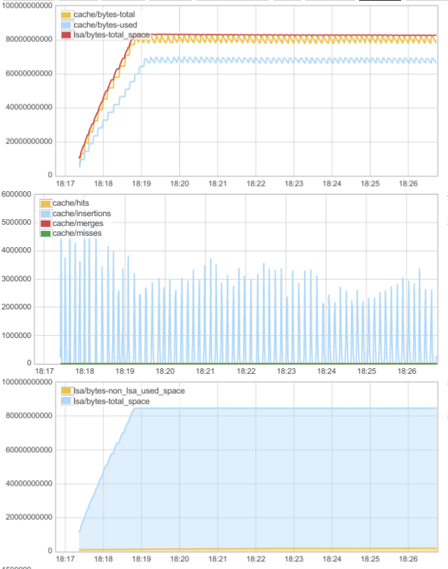
The graph in the bottom shows how the memory allocated by ScyllaDB is divided. lsa/bytes-non_lsa_used_space (yellow) shows the amount of memory allocated using seastar allocator, lsa/bytes-total_space (blue) shows memory reserved for the LSA allocator. We can see that while the yellow part remains constant, the blue part grows up to 80GB, and then also flattens out. This is because as the database is populated, data is inserted into memtables and later moved to cache, both of which are managed by LSA. The flattening-out is because we hit the memory limit and can’t cache any more.

On the middle graph we can see cache interactions. During the populating phase we see periodical spikes of cache/insertions. Those are flushed memtables moved into cache.

On the top graph we can see which fraction of LSA memory (red line) is dedicated to cache (yellow/blue). We can see that it’s mostly cache. The saw-like shape is caused by writes to memtables. First we see that while the red curve rises monotonically, the yellow curve has a stair shape. That’s because memtables receive data in uniform fashion, but are flushed periodically causing a rise in the cache memory. When memory is full, cache entries get evicted to make room for memtable data. That’s why yellow curve has a saw-shape after the red one reaches plateau.

Read workload

The test consisted of 7 instances of cassandra-stress started like this:

tools/bin/cassandra-stress mixed 'ratio(read=1)' duration=15min \
-pop 'dist=gauss(1..10000000,5000000,500000)' -mode native cql3 \
-rate threads=700 -node $SERVER

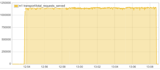
The image below shows how ScyllaDB behaves during the read workload over a 15 minute period. The Y axis represents CQL transactions per second. We can see how it does way beyond 1 million operations per second.

We can see how the workload interacts with the cache on the following graph:

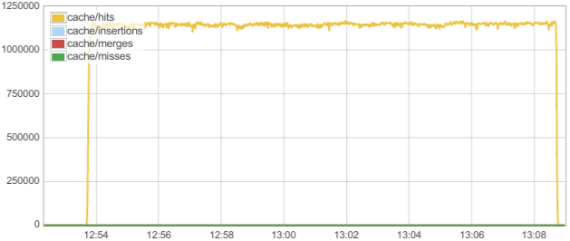
We can clearly see that all or almost all requests are served from cache.

Below is a flame graph generated for one of the CPUs on which ScyllaDB runs during the test:

Write workload

The test consisted of 7 instances of cassandra-stress started like this:

tools/bin/cassandra-stress write duration=15min -mode native cql3 -rate threads=700 -node $SERVER

Let’s look at the memory and cache statistics during the test:

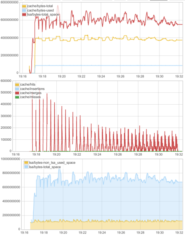
From the cache activity graph (second from the top) we can see that we have no insertions but a lot of merges. This means that when data is moved from memtable to cache it is merged with existing partitions. That means we’re dealing with a workload with a lot of overwrites. From the top graph we can see that cache/bytes-used stays at the same level, while cache/bytes-total and lsa/bytes-total_space get perturbed by memtable applies and flushes. The “used” cache size stays at the same level because the working set fits in memory.

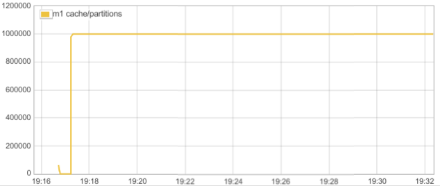
We can see that the partition count in cache remains constant (10^6):

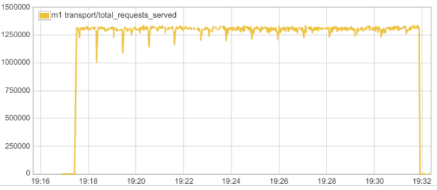
Let’s see what the throughput graph looks like. We can see we do about 1.3 million writes per second:

Below are disk activity statistics during the run:

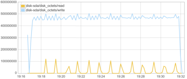
We can see high write activity, which can be attributed to commit log and sstable flushes.